24h在线客服


备案号:辽ICP备19007957号-1
![]() 聆听您的声音:feedback@highmark.com.cn企业热线:400-111-0321
聆听您的声音:feedback@highmark.com.cn企业热线:400-111-0321
Copyright ©2015- 海马课堂网络科技(大连)有限公司办公地址:辽宁省大连市高新技术产业园区火炬路32A号创业大厦A座18层1801室
The Impact of Monetary Policy on the Stock Market: An Empirical Study of China
This study emphasizes on the investigation about how the stock market responds to the fluctuations in the monetary policy in China. The dissertation employs narrow (M1) and broad money supply (M3) and the interest rate as the proxies of the monetary policy of China. Other two macroeconomic variables: inflation rate and exchange rate are also considered by this study. The dataset used in this dissertation covers the period from March 2005 to March 2014 in the monthly form.
Under the VAR models, the significantly positive effect of interest rate on the stock market returns is delayed for four months, while the significantly negative effect of the inflation rate and of the broad money supply are delayed for six and four months, respectively at the significance of 5%. Other variables present the insignificant influence on the returns of the Shanghai stock market. However, with the examination of the Shenzhen stock market, no significant correlation is identified between the stock market returns and its explanatory variables at the critical level of 5% in this dissertation.
In addition, both shocks in one standard deviation to the inflation rate and to the broad money supply demonstrate the negative influence on the stock market in the short term, while the shocks to the interest rate decrease the stock market returns in short term while in long term it shows the positive influence. More specifically, the current and delayed shocks in the Shanghai stock market explain a primary proportion of its movements. But the shocks of interest rate, inflation rate and the money supply account for a small proportion of the stock market returns movement.
Chapter one begins with the background of the research topic about the response of stock market to the monetary policy in China. It follows the study goals and the detailed research questions of this dissertation. The significance and a brief introduction of methodology of this thesis are also presented. At the end of this chapter, the organization of the dissertation is outlined.
According to Hafer and Hein (2007), capital market has played a crucial role in the economic growth and the expansion of business. As vital part of capital market, stock market brings about a bridge between the corporations and investors: corporations issue shares to raise capital and investors invest their money in stock markets. More importantly, the interaction between the return of stock market and monetary policy has attracted the attentions of academic world for a long period (Parrado and Velasco, 2001).
On the one hand, monetary policy is the tool utilized by central banks to assist the achievement of national economic objectives. Monetary policy affects the availability and cost of capital to adjust the consumption demand and investment trend, which show the impacts on stock market (Bernanke, Smith and Abel, 2003). On the other hand, there are a wide variety of approaches to launch the effective monetary policy by central banks, including inflation and money supply. Inflation is both a product and determinant of monetary policy, influences a broad set of economic activities, including the impacts on the stock markets resulting from the decline in purchasing power of currency.
On the basis of the study of Bernanke and Kuttner (2005), the return of stock market reflects the macroeconomic conditions of nations. The fluctuation of stock markets is linked with the economic development. In the recent decades, scholars in economic and financial fields have demonstrated increasingly interested in the issue of whether monetary policy influences the return of stock markets. According to Mishkin (2007), the market efficiency hypothesis suggests that an efficient stock market absorbs and reflects all information available in the market. Thus, the changes in monetary policy would influence the movement of the stock market.
More specifically, Mishkin (2007) argues that the changes in monetary policy will affect the discount rate or the risk premium required by investors, which in turn influences the assets price in stock markets. For instance, the changes in monetary policy like the decline in interest rate will promote the consumption and investment and hence contribute to the future value of assets and their growth. In addition, the reduction in interest rate devalues the bond price and attracts investors to invest in common shares. This results in the improvement in performance of stock markets.
Investors are not the only ones who concern about the response of stock market to the changes in monetary policy. Politicians also present same interest on the interaction. This is because monetary policy affects the assets price and because the learning of interlink contributes to the effective utilization of monetary policy as a tool to help promote the national economic goals (Bernanke and Kuttner, 2005). In other words, central banks implement the proxies of monetary policy to influence the economic activities.
China, as the largest developing economy, has experienced the dramatic growth in the past decade. In China’s process to transform the planning economy to market oriented economy, the Shanghai Stock Exchange and the Shenzhen Stock Exchange were established in 1990 and in 1991, respectively. There are A shares and B shares in both stock exchanges. A shares are traded for domestic investors only while B shares are for foreign investors. As the national economy of China moves towards market oriented deeply, the power of government regulation has still remained strong. This suggests that the response of stock market to monetary policy is worthy of detailed investigation. It is evident that the policy of government especially the monetary policy has a significant power over the national stock market.
With the respect of the existing literature, the studies about the influence of monetary policy on the return of stock market show mixed results. For instance, studies of Flannery and Protopapadakis (2002) and Bredin and his colleagues (2007) confirm the negative response of stock market to the changes in monetary policy. Other studies such as Rangel (2011) and Serwa (2006) identify the insignificant influence of the monetary policy on the return of the stock market. Among the existing literature, the debate about this controversial effect has been hot and immerse. There is no consensus on the response of stock market to the changes in monetary policy. The results about the issue are not only mixed but sometimes contradicting with others. In addition, the current literature mainly pays attention to the advanced stock markets, such as the U.S. market and the UK market while limited researches put their eyes on the developing countries especially China. The consequences of all motivate the author of this dissertation to devote efforts into the investigation of how the Chinese stock market responds to the changes in monetary policy.
The primary goal of this dissertation is to examine whether the stock markets of China respond to the changes in monetary policy. More specifically, the dissertation employs narrow and broad money supply and the interest rate as the proxies of the monetary policy of China. Besides the influence of the proxies of the monetary policy on stock market, other macroeconomic variables like inflation rate and exchange rate demonstrate impact on the stock markets. Through interpreting the findings, this dissertation aims to provide indications about the degree of monetary changes that affect the development of stock markets. The specific research questions of this thesis are summarized in the following table.
Table 1 Specific Research Questions of This Dissertation
|
Research Question 1 |
How the stock market of China responds to the change in the narrow money supply? |
|
Research Question 2 |
How the broad money supply influences the stock market of China? |
|
Research Question 3 |
Whether the fluctuation in interest rate affects the performance of stock market? |
|
Research Question 4 |
Whether stock market of China responds to the inflation? |
|
Research Question 5 |
Whether the exchange rate influences the stock market of China? |
The focus of this research is on the response of stock markets to the monetary policy in China. Many researches pay attention to the influence of monetary policy on the expected return of stock market. However, they focus on the impact of monetary policy on the daily returns of stock market. Few of the existing literature concentrate on the relatively long term effect of monetary policy on stock markets. This dissertation investigates the responses of both the Shanghai Stock Exchange and the Shenzhen Stock Exchange to the variation of Chinese monetary policy. In addition, the thesis employs the updated data to investigate the controversial issue. This dissertation tries to help expand the existing literature. In this way, this study makes contribution to the fruitfulness in the field of monetary economics.
On the basis of the current literature, the most widely used econometric model to examine the influence of monetary policy over the stock market is the vector autoregression model (thereafter, VAR). The VAR is associated with high flexibility to explore the time series dataset. In this research, it follows the approach of the previous studies to implement the VAR as the model to test how stock markets interact with the proxies of the monetary policy in China. In order to capture the effect and fully understand the issue, the impulse response functions and variance decompositions are used to examine the variance in the VAR modeling.
This dissertation focuses on particular stock markets in China, which include Shanghai stock market and Shenzhen stock market. The investigation is based on the sample of a series of variables, consisting of the proxies of monetary policy, inflation, exchange rate and returns of stock exchange from March 2005 to March 2014. Two empirical models, which focus on the Shanghai stock market and Shenzhen stock market respectively, are performed in this dissertation. More specifically, the first model focuses on the Shanghai stock market and the second one concentrates on the Shenzhen stock market in the sample period.
The typical organization of a thesis is suggested by the study of Perry (1998). Under the suggestion of Perry (1998), this dissertation is divided into five individual parts. Figure 1 outlines the structure of the present study.
Figure 1 Organization of the Present Study

Chapter one provides a basic overview of the entire dissertation. It begins with the background of the research problems. Then it describes the primary aim of the thesis and detailed research questions. The significance and the scope of the present study are presented as well. In addition, a brief of methodology and how the dissertation is organized are presented.
Chapter two emphasizes on the review of relevant literature about the response of stock markets to the change in monetary policy. Both the reviews of theoretical aspects and of the empirical studies in this field are covered. The testable hypotheses are developed on the basis of literature overview. A summary of this chapter is demonstrated at the end.
Chapter three depicts the research method of the present study. The process of data collection and research design are given in this chapter. The variables and empirical models are also described in depth.
Chapter four presents the empirical findings of the present study. It includes the analysis of the data characteristics and the VAR models. The results of impulse response functions and variance decomposition of models are explained after the VAR modeling.
Chapter five firstly provides a summary of the main findings. Then it describes the limitations of the present study and provides the suggestions about the future research directions.
Chapter two covers the review of relevant literature about the research theme. This chapter is divided into two main subgroups: the theoretical perspectives and the review of the empirical studies. At the end of chapter two, a summary of literature review and hypotheses are presented.
According to Brigham and Ehrhardt (2013), the beginning of the interpretation about the stock market is traced back to the study of Fisher (1930). Brigham and Ehrhardt (2013) suggest that the price of capital assets reflects the conditions of real economy of countries. They explain the study of Fisher (1930) by stating that capital assets indirectly contribute to the production of economy through the investment in the real economy. The capital assets in sufficiently advanced countries could be used to fight against the unexpected fluctuation of asset price. The argument of Fisher is called Fisher’s generalized hypothesis. Under the hypothesis, investors can convert their capital assets into real assets when assets price is expected to increase. In this situation, the price of capital assets indicates the expected fluctuations and they are positively associated (Ioannides et al., 2005).
Another important relevant theoretical perspective is the money demand function of Friedman (1956; cited in Choudhry, 1996). The study of Friedman investigates the interaction among the interest rate, the money supply and the return of stock markets. Friedman explains that the decisions of investors are highly dependent on the “consumption- saving decision”, which is influenced by the forecasting of the interest rate. The amount of money that investors decide not to consume today is the amount of investment available. The choice of consumption today or in the future is based on two criteria. First of all, the nature of investors’ utility and “indifferent curve” affects their choice of consumption today or in the future. Secondly, the analysis of trade-off between consumption today and consumption in the future could be perceived. Thus, the “consumption- saving decision” is about the money supply for investment, which is significantly influenced by the interest rate. In other words, whether to defer the consumption is highly associated with the return of the investments.
This suggests that the interest rate is an important factor that affects the “consumption- saving decision”. However, the argument of Friedman was challenged by the school Keynesian economists. In response, the monetary economists remodeled and then explained the argument of Friedman. According to Long (2000), the main critique of the theory is the unstable circulation speed of money. Thus, the association between the money supply and the assets price is controversial or non-existed. Under the aggregate supply function of Keynesian school, the money supply is dependent on whether the investors have only one option of remaining the bonds. The problem is that Keynesian theory focuses on the aggregate output rather than the price level. They believe that the monetary policy affects the interest rate and the interest rate influences the decisions of investors and finally impacts the economic outputs through a series of channels.
According to Cetin et al. (2004), the arbitrage pricing theory (thereafter, APT) recognizes the effect of macroeconomic variables over the return of capital assets. They implemented a series of macroeconomic variables to explain the response of stock markets. The macroeconomic variables covered in their study include inflation, output of industry, the price of oil, the risk premium, the consumption and the stock market return. The non-correlation among the macroeconomic variables and the returns of stock markets is assumed in their study. Their final findings confirm the significant correlation between the macroeconomic variables and the returns of stock markets. In other words, under APT, there is a linear correlation among the macroeconomic variables and the returns of stock markets. In addition, APT is appropriate to identify a set of risk factors, including inflation, interest rate and so forth. The following function presents the relationship:
R = E (r) + 
Where r is the return of stocks, is the parameter of stocks. The return of stock markets is related to the future expectation about the risks. In addition, Issing (2009) argues that the higher price of stocks reduces the cost of capital and in turn promotes the increase in investments.
In addition, according to Brigham and Ehrhardt (2013), the market efficient hypothesis is also related to the interaction between returns of stock market and the changes in monetary policy. The market efficient hypothesis suggests that the price of stocks should reflect all information available in the market if the stock market is efficient but the APT argues a linear correlation among the macroeconomic variables and the returns of stock markets. Furthermore, the General Equilibrium model by Tobin (1969, cited in Brigham and Ehrhardt, 2013) provides an alternative to examine how the stock market responds to the monetary policy. Tobin’s approach also identifies the significant interaction between the growth of money supply and budget deficit and the returns of stock market. Aliyu (2011) argues that the presence of stock market as a channel for central banks to employ monetary policy to influence the real economy of nations.
With the respect of the existing literature, the studies about the influence of monetary policy on the return of stock market show mixed results. Moreover, the current literature implements different econometric models to examine how the stock market moves regarding the changes in monetary policy.
Chaudhuri and Smiles (2004) adopt the research method of Johansen (1991) to explore how the stock market of Australia corresponds to its monetary policy. In their study, the broad money supply (M3) is used as the proxy of monetary policy. The macroeconomic variables consist of the household consumption, the gross domestic product (thereafter, GDP), and the commodity index of oil during the sample period from 1960 to 1998. More specifically, they confirm a significant long- run interaction between the stock returns in Australian market and its relevant monetary policy. The econometric model used by Chaudhuri and Smiles (2004) is the vector error correction model (thereafter, VECM).
Ga et al. (2006) use the stock market of New Zealand as a research objective. The monthly data from the beginning of 1990 to 2003 was used in their study. They adopt the VAR to analyze the dataset. In their research model, they include a series of variables, such as the long-term and the short-term interest rate, the inflation rate, the GDP of the country, the exchange rate, the price of oil and so forth. Similar to the study of Chaudhuri and Smiles (2004), they also find the long- term association of stock returns of New Zealand with its monetary policy proxies. However, only three factors: the narrow money supply (M1), interest rate and the GDP significantly relates to the stock market returns of New Zealand.
The study of Huashu and Yue (2003) devotes their efforts into Chinese stock market. They adopt the VAR as the econometric model to investigate the response of stock markets to the fluctuations in monetary policy. Their study covers a wide range of variables to test the association. Similar to the previous study, they also define the monetary policy as the interest rate and the money supply. But they only emphasize on the narrow money supply. The results of their study suggest the limited effect of the exchange rate and non-influence of the interest rate on the returns of Chinese stock exchange. However, the narrow money supply does significantly influence the returns of Chinese stock market. The relationship identified by them between narrow money supply and stock returns is the long term interaction.
Gregoriou et al. (2009) investigate the British stock market. Their study uses the bank rate from Bank of England as the proxy of monetary policy in the UK and tests how the changes in the bank rate would affect the returns of the British stock market. Under GMM approach, they find that the changes in bank rate lead to the corresponding movements in the returns of the British stock market. The study of Berdin et al. (2009) also reflects the similar results. But they test how the composite index as well as the sixteen industries index responds to the fluctuations of the bank rate of Bank of England. The study confirms the negative association and the different degree of the monetary policy’s influence on the different industries in the UK.
The study of Hassan and Javad (2009) is based on the sample of Pakistan from 1998 and 008. The monthly data is adopted by them to investigate how the stock returns of Pakistan stock markets correspond to the monetary policy. Their study provides the evidence about the presence of the short- term effect of monetary policy on the returns of stock market. According to the results of Granger causality analysis, they confirm the presence of bidirectional causality between monetary policy and the returns of stock market in Pakistan in the short run. The similar findings are found by Yu (1997), who performed research in Japan security market. In addition, the study of Yu (1997) further identifies the bidirectional causality moving from the returns of stock market to the exchange rate in the short run at Japan security market.
The study of Naceur et al. (2007) expands their research scope to eight countries, including “Morocco, Oman, Turkey, Egypt, Tunisia, Saudi Arabia, and Bahrain”. The VAR model is also adopted in their study. Their findings are summarized as the following: 1) they identify the statistically significant interaction of stock returns with the monetary policy in Bahrain, Oman, Jordan and Saudi Arabia; 2) the influence of monetary policy in the previously mentioned countries is more significantly than that in Tunisia and Morocco; 3) only Jordan and Saudi Arabia perceive the bidirectional interaction running from the monetary policy proxies to stock returns in the short term.
Ehrmann and Fratzscher (2004) concentrate on how the daily returns of individual firms are influenced by the monetary policy. They follow a distinctive approach to differentiate their study from the existing literature. They divide the 500 individual firms into nine industrial sectors as well as sixty industry groups during the period of 1994 to 2003. After these preparations, they make a conclusion that the capital intensive sectors significantly, negatively react to the changes in the proxies of the monetary policy in the United States. In addition, they also find that corporations with high financial constraints are more likely to be influence by the monetary policy than those with low financial constraints.
The study of Serwa (2006) devotes his efforts into an emerging stock market – Poland. Serwa (2006) only utilizes the interest rate as the indicator of the monetary policy and investigates the response of Poland stock market to the monetary policy measure. In addition, Serwa (2006), on the basis of heteroscedasticity methodology, analyze the data from 1999 to 2005 in the daily form. The results of his study suggest that the response of Poland stock market is negatively correlated with the changes in the monetary policy at their announcement day. However, the short term relationship is insignificant.
Afzal and Hossain (2011) confirm both the long-term and short –term interaction moving from monetary policy to the proxies of monetary policy. More specifically, they utilize the narrow money supply (M1), the interest rate and the exchange rate to represent the monetary policy of Dhaka. They find out the unidirectional association among the stock returns, the exchange rate, and the narrow money supply. When they adjust their model into bivariate VECM, they identify the long run causality moving from the narrow money supply to the returns of Dhaka stock market. In addition, their study gets an insignificant link between the returns of Dhaka stock market and the inflation rate.
The study of Berrument and Kutan (2007) is very interesting. They emphasize on how long the influence of monetary policy on the returns of stock market would disappear. They pay their attention to the Turkey market with a sample period from 1980 to 2007. Under the VAR model, they find the significant interaction between the returns of stock market and the monetary policy. However, ranging from 9 months to 24 months, the influence resulting from the monetary policy disappears. In addition, the speed of disappearance is closely associated with the selection of stock index. From this perspective, they make a conclusion that there is no association between stock returns and monetary policy in the long term while the short term correlation does exist.
Bernanke and Kuttner (2005) make their study distinctive from other studies since they emphasize on the effect unexpected fluctuations in the monetary policy on the stock market. They state that the positive unexpected fluctuations in the monetary policy reduce the expected future returns and increase the real interest rate and raise the required risk premium. They also follow the VAR model to test the effect of monetary policy. They draw a conclusion that the expected future returns, the real interest rate and the required risk premium show the significant effect whereas the effect of the interest rate is unclear. The early study of Boudoukh and Richardson (1993) indicates the negative effect of inflation over the stock market. The negative effect results from the short term returns less than one year. But when they expand the data into a long time period such as 5 years in the annual form, they find a positive association between the inflation rate and the security market returns.
Schotman and Schweitzer (2000) devote their efforts into the investigation about how the inflation rate affects the stock market returns in different time horizons. In their study, they argue that the negative inflation reduces the risk of stocks in short term but the relationship transforms into positive sign when these researchers prolong their time horizon into ten years. The growth of inflation indicates the better returns of stock markets. The study of Engsted and Tanggaard (2002) also investigates how the inflation rate affects the stock market returns in different time horizons (e.g. one year, five years or ten years). They use the VAR model to make the investigation about the UK market, Danish market and the bond markets in both two countries. More specifically, they find that inflation rate slightly affects the returns of the UK market under each time horizon. However, in Danish stock market, the significance of the relationship increases when the time horizons expand. Their study shows the similarity with that of Boudoukh and Richardson (1993).
In addition, Wong and Wu (2003) extend their research scope by including G7 countries and eight countries in Asia to examine the Fisher effect both in the long run and in the short run. They obtain a more significantly positive correlation between inflation rate and stock market returns when they use GMM method than when they implement the ordinary least square method in different time horizons. Furthermore, the study of Kim and In (2005), which follows the wavelet scaling method to analyze the data ranging from 1926 to 2006, find that the inflation rate positively correlates with the stock market returns in the long run but demonstrates the negative association in the short time period. Their study also supports that of Boudoukh and Richardson (1993).
The U.S. security market is focused by Hamrita and Trifi (2011). Their data is in the monthly form and covers the period from 1990 and 2008. Different from other studies, they adopt a different methodology to examine how the stock market corresponds to the monetary policy changes. The methodology used by them is called wavelet transform. Under this methodology, they find a long term relationship between these two variables. But their study highlights the presence of non-linear correlation between the stock market returns of the U.S. and the exchange rate.
Under the bivariate EGARCH model, the study of Qayyum and Anwar (2011) finds that the repo rate of banks shows the significant influence on the stock market. The interesting point of their study is the assumption made by them. Before their analysis, they assume that the stock return of Pakistan is kurtic instead of following the normal distribution. Moreover, they also confirm that the fluctuation of the monetary policy places the significant influence on the returns of Pakistan stock market. But the controversy in their study is located in the credit of their assumption about the kurtic returns of Pakistan stock market.
On the basis of reviewing the existing literature, this dissertation finds that the mainstream of studies follows the VAR model to test how the stock market responds to the changes in the monetary policy. The measures of the changes in the monetary policy used by the existing literature include the interest rate, both the narrow money supply (M1) and broad money supply (M3). The exchange rate is also considered as a macroeconomic variable. The monthly return of Shanghai Stock Exchange as well as of Shenzhen Stock Exchange is used in this dissertation for two empirical models. The present study also follows the most widely used model VAR to examine the relationship and utilizes the interest rate, both the narrow money supply (M1) and broad money supply (M3), and the exchange rate as the proxies of the changes in the monetary policy.
One of the important features of the VAR model is that it imposes little economic structure on the analysis. Thus, the underlying economic structure is less relevant. This is very important in this study since China, as an emerging economy, is characterized by uncertainties and abnormalities within the economic structure. The other benefit of the use of the VAR model refers to the inclusion of the “endogeneity - the interdependence” among a vector of variables.
According to the examination of the previous literature, the present study develops the following hypotheses that will be tested. Table 2 summarizes the hypotheses testable in this dissertation.
Table 2 Hypotheses of the Dissertation
|
Hypothesis |
Expected Sign |
|
|
Hypothesis 1 |
positive |
The narrow money supply positively correlates with the Chinese stock market returns |
|
Hypothesis 2 |
positive |
The broad money supply positively correlates with the Chinese stock market returns |
|
Hypothesis 3 |
negative |
The interest rate is negatively associated with the Chinese stock market returns |
|
Hypothesis 4 |
positive |
The inflation rate is positively associated with the Chinese stock market returns |
|
Hypothesis 5 |
Negative |
The exchange rate is negatively associated with the Chinese stock market returns |
As indicated in the previous sections, the measures of monetary policy in China are money supply and interest rate. The study of Stonecash et al. (2011) points out that the greater money supply and low interest rate indicates the expansionary policy and will stimulate the economic growth. But, in contrast, low money supply and high interest rate indicates the contractionary policy, which cools down the economy. Thus, the expected sign of the interest rate is negative whereas that of the money supply is positive. The review of literature also indicates the possibility of negative association between the exchange rate and stock market returns but of the positive association between the inflation rate and the stock market returns.
Chapter three demonstrates the research methodology in depth. In the first step, this chapter introduces the depiction of variables in this dissertation. Then the model specification is presented. In the following, the diagnostics test will be described in short as well.
With the effort to capture the response of stock market to the changes in monetary policy, the measures of the changes in the monetary policy include the interest rate and both the narrow money supply (M1) and broad money supply (M3). All the variables are transformed in the form of log, which are based on the previous literature dealing with the measurement of variables.
Money Supply
Money supply is one of the measures of the changes in monetary policy in this dissertation. The changes in money supply can affect the real economic activities. In order to remain the stable economy, central banks can adjust the amount of money supply to influence the real economy and hence the capital market. As mentioned before, the greater money supply and low interest rate indicates the expansionary policy and will stimulate the economic growth. But, in contrast, low money supply and high interest rate indicates the contractionary policy, which cools down the economy. The equations for the money supply are presented as the following:

Where t denotes the specific month at a specific year
Interest Rate
The change in interest rate has the impact on the economic activities and hence the cost of capital. In this way, the profits of individual firms will be affected by the interest rate, which in turns influences the stock returns. The formula to present the interest rate is shown:

The fluctuation of the money supply will result in the variation in the inflation rate, which shows the significant influence on the corporations’ profits and expense as well as the net present value of investments. On the basis of literature review, many researches include the inflation rate as one of the macroeconomic variables in the models that could justify the association between monetary policy and the stock market returns. In the present study, the inflation is also taken into consideration and the consumer price index (thereafter, CPI) is used as the measure of inflation in China. Thus, the equation for CPI is presented as the following:

With the consideration of China’s national conditions, Chinese government also implements the trade of foreign currency as the adjustment tool of monetary policy. In the present study, the effective exchange rate of Renminbi (thereafter, CNY) is utilized to capture its influence on the stock market returns. The equation for the CNY is in the following:

In Mainland China, there are two stock exchanges: Shanghai Stock Exchange established in 1990 and Shenzhen Stock Exchange established in 1991. In this research, the Hong Kong Stock Exchange is excluded with the consideration of the different ruling policy compared to the Mainland China. Therefore, in order to fully capture the response of stock market to the changes in monetary policy, this dissertation constructs two models to test the responses of these two stock markets, respectively.
Monthly returns of Shanghai Stock Exchange Index (thereafter, SSEI) and of Shenzhen Stock Exchange Index (thereafter, SZEI) are implemented as the stock market returns in this dissertation. More specifically, these two dependent variables are specified as the following two equations:

In addition, with goal to eliminate the seasonal effect of time series dataset, the present study introduces the 11 dummy variables. More specifically, the value of 1 represents a month and the value of 0 represents the other month.
The present study also follows the most widely used model VAR to examine the relationship between the interest rate and the narrow money supply (M1) and broad money supply (M3) (as the proxies of the changes in the monetary policy), and the macroeconomic variables including the exchange rate and inflation rate, and the stock market returns. Thus, the two estimated models are illustrated as the following:
Where
Focusing on the response of stock market to the monetary policy, the present study covers the time period from March 2005 to March 2014. Moreover, the data is used in monthly form. The total number of observation is 109. The data about the returns of two stock markets are retrieved from Yahoo Finance China. In the open database of Organization for Economic Co-operation and Development (OECD), narrow and broad money supply, interest rate and the CPI rate can be directly obtained and the exchange rate is obtained from the investing.com.
In this dissertation, the time series data is used to achieve the primary research goals. Before to perform the VAR model, the characteristics of time series data require the test about the data is stationary and cointegrated (Hamilton, 1994). More specifically, according to Hamilton (1994), there are four main types of stationary tests, including “Dikcey-Fuller (DF)”, “Augumented Dickey-Fuller (ADF)” and “Phillips Perron (PP)” test. These four types of the stationary tests are the most widely used by researchers in the field of time series studies. The present study adopts the ADF test to test the stationarity of the dataset since the ADF is simple to carry out and easy to understand. In addition, the ADF test has also been widely used in many of the empirical studies.
The null hypothesis of the ADF test (H0): the dataset is not stationary, which shows one unit root;
The alternative hypothesis of the ADF test (h3): the data set is stationary without one unit root.
On the other hand, the examination of the cointegration effect about the dataset can demonstrate whether there is the long term equilibrium between the dependent variables and the independent variables (Hamilton, 1994). The most widely used approach to test the cointegration effect is the Johansen cointegration test. The study of Agbola (2004) points out that the “Johansen cointegration tests a number of contegration vectors rather than a single one and hence increases the accuracy”. After the ADF test and the examination of the cointegration effect, the VAR model is used to test the association between the stock market returns and the monetary policy. In addition, all of the data analysis is carried out by Eviews version 7.2.
The empirical findings of this research are presented in chapter four. The descriptive statistics of variables are firstly analyzed. Then the ADF test and Cointegration test are performed in order. The third step is to present the findings resulting from the VAR models. At the end of the chapter, the results of impulse response function and variance decomposition are demonstrated.
The characteristics of all the variables in this dissertation are summarized in Table 2. There are total 109 observations in the present study. The average return of Shanghai Stock Exchange is 0.1764% in the sample period, which is slightly lower than that of Shenzhen Stock Exchange (0.4936%). The standard deviations of stock market returns suggest that the returns of Shanghai Stock Exchange are less volatile than those of Shenzhen Stock Exchange (S.D. = 0.038958 and S.D. = 0.042755, respectively). The average change in the interest rate is 0.2828% in the sample period with a standard deviation of 0.07824. The average movement of the inflation rate is 0.1019% with a standard deviation of 0.002595. The average fluctuation in the exchange rate is – 0.0114%.
The average changes in the narrow money supply and the broad money supply are 0.4936% and 0.5906%, respectively. But the change in the narrow money supply is more volatile than that in the broad money supply (S.D. = 0.004066 and S.D. = 0.002199, respectively). With the respect of Jarque- Bera test, almost all the p-value of variables except the stock market returns of Shenzhen Stock Exchange is statistically significant at the critical value of 5%. The result of Jarque- Bera test indicates that all of the variables in this dissertation except the stock market returns of Shenzhen Stock Exchange are not normally distributed at the significance level of 5%.
Table 2 Descriptive Statistics of the Variables in the Log Form
|
|
SSEI |
INR |
CPI |
CNY |
SZEI |
M1 |
M3 |
|
Mean |
0.001764 |
0.002828 |
0.001019 |
-0.00114 |
0.004596 |
0.004936 |
0.005906 |
|
Median |
0.003434 |
0.004572 |
0.000868 |
-0.00067 |
0.009584 |
0.005013 |
0.005532 |
|
Maximum |
0.105328 |
0.261675 |
0.011147 |
0.005985 |
0.110386 |
0.018457 |
0.013364 |
|
Minimum |
-0.12281 |
-0.3243 |
-0.00393 |
-0.00906 |
-0.11643 |
-0.00825 |
0.00139 |
|
Std. Dev. |
0.038958 |
0.07824 |
0.002595 |
0.002268 |
0.042755 |
0.004066 |
0.002199 |
|
Skewness |
-0.60542 |
-0.41773 |
0.559567 |
-0.46681 |
-0.49001 |
0.239308 |
1.434286 |
|
Kurtosis |
4.179113 |
7.502784 |
4.025666 |
5.573253 |
3.408771 |
4.913899 |
5.56149 |
|
Jarque-Bera |
12.97306 |
95.25267 |
10.46605 |
34.03195 |
5.120842 |
17.67655 |
67.17094 |
|
Probability |
0.001524 |
0 |
0.005337 |
0 |
0.077272 |
0.000145 |
0 |
|
Sum |
0.19226 |
0.308268 |
0.11108 |
-0.12425 |
0.500937 |
0.538012 |
0.643709 |
|
Sum Sq. Dev. |
0.163918 |
0.661129 |
0.000727 |
0.000556 |
0.197424 |
0.001786 |
0.000522 |
|
Observations |
109 |
109 |
109 |
109 |
109 |
109 |
109 |
(Source: prepared by the author in Eviews)
Figure 2 illustrates the trends of variables in multiple graphs. It can be seen from Figure 2 that the reaction of Shenzhen Stock Exchange to the financial crisis is much sensitive than that of Shanghai Stock Exchange. This also reflects the more volatility of Shenzhen Stock Exchange than that of Shanghai Stock Exchange. The change in the narrow money supply is sharper than that of the broad money supply in the sample period. In Figure 2, the fluctuation of the exchange rate is more evident after 2010. The changes in the interest rate and in the inflation rate are both very volatile from March 2005 to March 2014.
Figure 2 Trends of Variables in Log Form
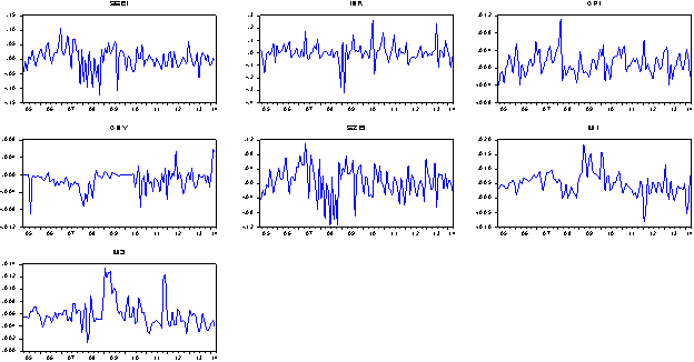
(Source: prepared by the author in Eviews)
Table 3 provides a summary of the correlation analysis among variables in this dissertation. The result of correlation analysis indicates that the inflation rate is positively corresponding to the returns of both two stock markets at the significance of 10%. Both the returns of both two stock markets are positively correlated with the narrow money supply and the broad money supply at the critical level of 5%. But the correlation analysis only involves in two individual variables not focuses on the overall effect of independent variables on the dependent variables in this dissertation. The following sections present the preliminary test and the VAR models in the present study.
Table 3 Correlation Analysis of the Variables
|
|
|
|
|
|
|
|
|
|
|
|
|
|
|
|
|
|
|
Correlation |
|
|
|
|
|
|
|
|
Probability |
SSEI |
INR |
CPI |
CNY |
SZEI |
M1 |
M3 |
|
SSEI |
1.000000 |
|
|
|
|
|
|
|
|
----- |
|
|
|
|
|
|
|
|
|
|
|
|
|
|
|
|
INR |
-0.008307 |
1.000000 |
|
|
|
|
|
|
|
0.9317 |
----- |
|
|
|
|
|
|
|
|
|
|
|
|
|
|
|
CPI |
0.178642 |
0.055342 |
1.000000 |
|
|
|
|
|
|
0.0631** |
0.5676 |
----- |
|
|
|
|
|
|
|
|
|
|
|
|
|
|
CNY |
0.139186 |
-0.130841 |
-0.101454 |
1.000000 |
|
|
|
|
|
0.1489 |
0.1751 |
0.2939 |
----- |
|
|
|
|
|
|
|
|
|
|
|
|
|
SZEI |
0.908587 |
-0.043112 |
0.194975 |
0.127176 |
1.000000 |
|
|
|
|
0.0000*** |
0.6562 |
0.0422** |
0.1876 |
----- |
|
|
|
|
|
|
|
|
|
|
|
|
M1 |
0.221496 |
0.029169 |
0.051434 |
-0.005483 |
0.229592 |
1.000000 |
|
|
|
0.0206** |
0.7634 |
0.5953 |
0.9549 |
0.0163** |
----- |
|
|
|
|
|
|
|
|
|
|
|
M3 |
0.198136 |
-0.092442 |
0.010324 |
0.099825 |
0.225807 |
0.583324 |
1.000000 |
|
|
0.0389** |
0.3390 |
0.9152 |
0.3017 |
0.0182** |
0.0000 |
----- |
|
|
|
|
|
|
|
|
|
|
|
|
|
|
|
|
|
|
(Source: prepared by the author in Eviews)
Note: “* stands for the statistical significance at 10%; ** stands for the statistical significance at 5%; and *** stands for the statistical significance at 1%”.
Before performing the VAR models, this dissertation has to conduct the preliminary tests to examine whether the data can be used for time series analysis. The following sections show the results of the ADF test and the Johansen cointegration test.
The dataset used in this dissertation is time series data so that there is a need to carry out the stationary test. More specifically, the present study adopts ADF method to test the stationarity of the data. The result of the ADF test is illustrated in Table 4. In Table 4, the variables included in the estimated models are all statistically significant at the critical level of 5%. The p-values of all variables (< 0.05) indicate that the null hypothesis of the ADF test must be rejected in this dissertation at the critical level of 5%. In other words, it is safe to draw a conclusion that all of the variables included in the estimated models are stationary. More importantly, the output of the ADF test suggests the possibility of long run association among variables.
Table 4 ADF Test of the Variables
|
Null Hypothesis: SSEI has a unit root |
|
|
|
|
|
|
|
||
|
Exogenous: Constant |
|
|
|
|
|
|
|
||
|
Lag Length: 0 (Automatic - based on SIC, maxlag=12) |
|
|
|||||||
|
ADF Test |
SSEI |
INR |
CPI |
CNY |
SZEI |
M1 |
M3 |
||
|
t-statistics |
-9.53878 |
-11.8499 |
-8.01161 |
-4.56606 |
-9.56754 |
-3.01712 |
-3.95453 |
||
|
Prob. |
0.0000*** |
0.0000*** |
0.0000*** |
0.0003*** |
0.0000*** |
0.0365** |
0.0024*** |
||
(Source: prepared by the author in Eviews)
Note: “* stands for the statistical significance at 10%; ** stands for the statistical significance at 5%; and *** stands for the statistical significance at 1%”.
4.2.2 Johansen Cointegration Test
Prior to the introduction of Johansen Cointegration test, the lag order of this dissertation has to be determined at the first place. “Akaike Information Criterion (AIC)”, “Schwartz Bayesian Information Criterion (SBIC)”, “Hanna and Quinn Information Criteria (HQIC)”, and “Final Prediction Error (FPE)” are the four most commonly used selection criteria of lag order (Hamilton, 1994). In addition, if these four selection criteria contrast with each other, the “Likelihood Ratio (LR)” can be also used to make the lag order selection. The lag order with minimum values of the four criteria and the LR should be the one used in this dissertation. Table 5 and Table 6 in the Appendix present the results of lag selection for the two estimated models in the dissertation. It is evident in Table 5 and Table 6, the lag length of 6 should be chosen for the further research procedures because it contains the minimum values of the LR since four selection criteria do not reach an agreement.
After the selection of lag length, the Johansen Cointegration test is performed for two estimate models mentioned in the chapter 3 (equation 9 and equation 10, respectively). As examined in the section 4.2, all of the variables included in the estimated models are stationary, which suggests the possibility of long run association among variables. Moreover, if the effect of cointegration was confirmed, the short term shocks among the relationship between the stock market returns and the proxies of the monetary policy and the macroeconomic economics would be corrected in the long time horizon.
Table 7 and Table 8 summarize the results of Johansen Cointegration examination estimated model 1 and estimate model 2, respectively. The comparison between the value of trace statistics and 0.05 critical values can tell whether the effect of cointegration exists. In model 1, all levels of trace statistics are higher than 0.05 critical values except level 4, suggesting that there would be single cointegration at least for a vector of variables. In model 2, all of the trace statistics are higher than 0.05 critical values. This also indicates that there would be single cointegration at least for a vector of variables.
Table 7 Johansen Cointegration Test of the Estimated Model 1
|
Hypothesized |
Trace |
0.05 |
|
|
|
No. of CE(s) |
Eigenvalue |
Statistic |
Critical Value |
Prob.** |
|
None * |
0.328101 |
122.7542 |
95.75366 |
0.0002*** |
|
At most 1 * |
0.263543 |
81.39881 |
69.81889 |
0.0045*** |
|
At most 2 * |
0.173208 |
49.58474 |
47.85613 |
0.0341** |
|
At most 3 * |
0.138422 |
29.80373 |
29.79707 |
0.0499** |
|
At most 4 |
0.081171 |
14.30876 |
15.49471 |
0.0748* |
|
At most 5 * |
0.051553 |
5.50465 |
3.841466 |
0.019** |
(Source: prepared by the author in Eviews)
4.3 Findings of the VAR Models
The following sections present the output of two estimate models in this dissertation: one is for the Shanghai stock market and the other is for the Shenzhen stock market.
4.3.1 Empirical Results of Estimate Models
The preliminary test of the data shows that the data is stationary and the cointegration effect exists. Thus, the VAR model is used to examine the relationship between the interest rate and the narrow money supply (M1) and broad money supply (M3) (as the proxies of the changes in the monetary policy), and the exchange rate and inflation rate, and the stock market returns. Moreover, the lag length used in the equation 9 (model 1) is 6 (see Table 5 in the Appendix), which is based on the criteria of the LR criteria. Thus, the optimal lag length for this dissertation is lag 6 (six months). The result of the VAR estimated model 1 is presented in Table 9 in the Appendix.
In the present study, only the interest rate and the narrow money supply (M1) and broad money supply (M3) are viewed as the proxies of the changes in the monetary policy in China. The focus of this study is to evaluate the effect of monetary policy on the returns of Shanghai Stock Exchange. The critical value of t-distribution at 5% with the freedom degree of 102 is around the absolute value of 1.660. This critical value of 1.660 is used to justify whether the correlation between monetary policy variables and the market stock returns is statistically significant. Therefore, through the comparison between the absolute value of 1.660 and the t-statistics in the first column in Table 9, this dissertation can identify whether the monetary policy in China has impact on the returns of Shanghai Stock Exchange Index.
The result of model 1 (see Table 9 in the Appendix) reflects that only the interest rate of the four lagged month (INR (-4)), the inflation rate of the six lagged month (CPI (-6)), and the broad money supply of the four lagged month (M3 (-4)) are significantly correlated with the returns of Shanghai Stock Exchange Index at the critical value of 5%. The rest of variables are not statistically at the critical value of 5%. More specifically, the stock market responded to the changes in monetary policy after either four months or six months. In addition, the effects of the interest rate and the broad money supply on the stock market returns have the fastest speed in this dissertation. But its effect is also delayed for four months after the changes occurred in the monetary policy. The effect of inflation rate on the stock market returns is delayed for half a year after the changes occurred in the monetary policy. However, the lagged changes in the exchange rate and in the narrow money supply do not demonstrate delayed influence on the stock market returns.
Comparing with the inflation rate, the adjustments in the interest rate and the broad money supply are more efficient as the monetary policy than the adjustments of the inflation rate, which influences the stock market returns. The insignificant effect of the lagged exchange rate on the stock market returns might attributed to the fact that the exchange rate regime is still under the control of the central bank. It is not as free floated as the expectation. This finally attributes to the special economic conditions of China although China has increasingly become market oriented. But the government has still played a dominated role in the capital market. However, in the VAR model, the interpretation of the model 1 shows that the exchange rate does not give the real response of the stock market.
With the respect of Shenzhen stock market, the results are quite controversial. The output of estimate model 2 is presented in the Table 10 in the Appendix. When comparing to the absolute critical value of 1.660, this dissertation does not identify any significant association between the stock market returns of Shenzhen and the monetary policy proxies and the macroeconomic variables at the critical significance of 5%. On the basis of the empirical findings of Shenzhen stock market, it is hard to determine whether the stock market responds to the changes in the monetary policy or conclude whether there is long run association between them.
In addition, the different signs of the lagged values of the significant variables in both models suggest the easiness of identifying the exact relationship between the stock market returns and the monetary policy in the long term. More specifically, INR (-4) shows the significantly positive influence on the stock market returns while CPI (-6) and M3 (-4) illustrate the significantly negative influence on the stock market returns. Furthermore, this dissertation determines to carry out the Impulse Response Functions (thereafter, IRFs) and Variance Decompositions (thereafter, VDCs) to assess whether the short term shocks are corrected in the long term horizon. More specifically, the sharp short term fluctuations in the monetary policy might influence the stock market returns in China. With the consideration of this issue, the present study decides to apply the IRFs and VDCs to analyze the influence of the sharp shocks in the monetary policy on the stock market returns in China. Furthermore, the VDCs help to identify whether the random innovation of information presents the impacts on the stock market returns in China. The following sections present the output of IRFs and VDCs, respectively.
4.3.2 Impulse Response Function
Figure 3 presents the output of IRFs at the one standard deviation random shock, showing that one standard deviation random shock of the stock market returns responds to a series of variables identified in this market. Due to the insignificance of all variables in the estimate models, only the IRFs of the Shanghai stock market are performed in this dissertation. In Figure 3, the x axis presents the time period in months, where 1 denotes one month and 2 denotes two months. The rest is in the same manner. The y axis is response of the stock market returns to the monetary policy variables as well as the macroeconomic variables.
In Figure 3, it can be seen that a one standard deviation shock to the interest rate decreases the stock market returns and it starts to increase finally demonstrating an increase in the stock market returns after five months of the shock. But then the stock market returns decrease to the previous level about 9 months after the shock. With the respect of CPI, its one standard deviation shock leads to the decrease in the stock market returns starting from the one month. Around ten months after the one standard deviation shock, the response of the stock markets returns covers aback to its previous level and begins to go up.
Regarding the exchange rate, its one standard deviation shock leads to the decrease in the stock market returns during the period of six months and then it begins to rise from the seven months after the shock. For the narrow money supply, it leads to the decrease in the stock market returns in the three months and begins to increase during the three months to four months. But after four months, it deteriorates the stock market returns again. In addition, with the respect of the broad money supply, there is no effect of one standard deviation shock on the stock market returns in the first three months. After three months of the shock, it begins to increase the stock market returns but then decrease in the five months and six months.
Figure 3 Response of SSEI to Variables at One Standard Deviation
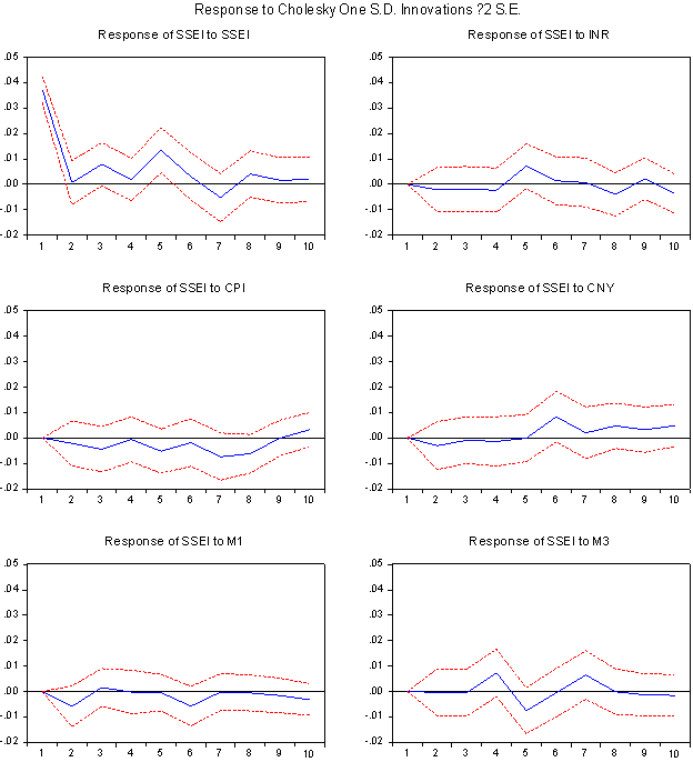
(Source: prepared by the author in Eviews)
4.3.3 Variance Decomposition
VDCs is another way widely used in the empirical researches to estimate the extent to which the stock market returns responds to its own shocks and to the shocks of the monetary policy variables and the macroeconomic variables. In other words, this approach decomposes the variance of the stock market returns that is caused by the random innovation information available in the stock market. Different from the IRFs, which emphasizes on the response of dependent variables to the shocks of independent variables, VDCs focus on the decomposition of variance. In this way, VDCs helps this dissertation to test the impact of random innovation on the stock market returns. The result of VDCs is presented in the Table 11. The graphic form is presented in the Figure 4 in the Appendix.
It is evident in the Table 11 that the shocks in the Shanghai stock market explain more than 72% in the ten periods. But the shocks in the interest rate only explain a small proportion of the shocks in the Shanghai stock market with a maximum of around 4% in the ten periods. Similarly, the shocks of the inflation rate as well as of the exchange rate explain around 6% of the variance of the Shanghai stock market returns in the ten periods. The shocks of the narrow money supply only account for 3% of the variance in the stock market returns in the ten periods. In contrast, the shocks of the broad money supply only account for around 6% of the variance in the stock market returns in the ten periods. However, only the current stock market returns shocks and the delayed shocks show the significant effect on the future stock market returns while other shocks of the monetary policy variables and the macroeconomic variables show limited effect. Along with the result of IRFs (see Figure 3 in section 4.3.2), the stock market returns of Shanghai respond to the changes in the fluctuations in the monetary policy.
Table 11 Variance Decomposition of SSEI
|
|
|
|
|
|
|
|
|
|
|
|
|
|
|
|
|
|
|
Period |
S.E. |
SSEI |
INR |
CPI |
CNY |
M1 |
M3 |
|
|
|
|
|
|
|
|
|
|
|
|
|
|
|
|
|
|
|
1 |
0.037284 |
100.0000 |
0.000000 |
0.000000 |
0.000000 |
0.000000 |
0.000000 |
|
2 |
0.037999 |
96.30690* |
0.330225 |
0.335213 |
0.656712 |
2.363356 |
0.007593 |
|
3 |
0.039151 |
94.74666* |
0.558732 |
1.613918 |
0.674917 |
2.385109 |
0.020668 |
|
4 |
0.039962 |
91.15204* |
0.859089 |
1.571769 |
0.768456 |
2.293250 |
3.355400 |
|
5 |
0.043706 |
85.55283* |
3.350270 |
2.737864 |
0.643164 |
1.927040 |
5.788829 |
|
6 |
0.045025 |
81.07252* |
3.252779 |
2.747590 |
4.011517 |
3.448878 |
5.466720 |
|
7 |
0.046433 |
77.50097* |
3.079794 |
5.133820 |
3.962109 |
3.245870 |
7.077437 |
|
8 |
0.047437 |
74.97961* |
3.654999 |
6.664810 |
4.796082 |
3.123461 |
6.781041 |
|
9 |
0.047670 |
74.35739* |
3.834688 |
6.600051 |
5.204186 |
3.205586 |
6.798096 |
|
10 |
0.048335 |
72.47394* |
4.331694 |
6.861013 |
6.063224 |
3.556016 |
6.714112 |
|
|
|
|
|
|
|
|
|
|
|
|
|
|
|
|
|
|
|
|
|
|
|
|
|
|
|
(Source: prepared by the author in Eviews)
4.4 Discussions
In this dissertation, the ADF test and the Johansen Cointegration test suggests that the possibility of long run association among variables and that the short term shocks among the relationship between the stock market returns and the proxies of the monetary policy and the macroeconomic economics would be corrected in the long time horizon. The results of ADF test and the Johansen Cointegration test also justify the application of the VAR model in this dissertation.
With the respect of Shanghai stock market, the effect of the interest rate on its returns is delayed for four months (INR (-4)), the effect of the inflation rate on its returns is delayed for six months (CPI (-6)), and the effect of the broad money supply is prolonged for four months (M3 (-4)). Only INR (-4), CPI (-6) and M3 (-4) are statistically significantly associated with the stock market returns at the critical level of 5%. However, the rest of the variables remain the insignificant impact on the Shanghai stock market. In other words, the significant long term relationship between the stock market returns and the interest rate, inflation rate and the broad money supply could be identified in this dissertation. More specifically, INR (-4) shows the significantly positive influence on the stock market returns while CPI (-6) and M3 (-4) illustrate the significantly negative influence on the stock market returns. The identification of the long term relationship between the stock market returns and the changes in monetary policy is constant with the studies of Chaudhuri and Smiles (2004), Ga et al. (2006), Huashu and Yue (2003), Gregoriou et al. (2009), and Berdin et al. (2009), which all find the long run association.
Regarding the hypotheses developed in this research, the hypothesis 1 and hypothesis 5 could not be rejected since there is no influence of the narrow money supply and the exchange rate on the stock market returns. The Hypothesis 3 is supported by the findings that INR (-4) shows the significantly positive influence on the stock market returns. The hypothesis 2 and hypothesis 4 are also supported by the findings but the signs of the relationship (negative) are opposite from the expectation (positive).
In addition, the effects of the interest rate and the broad money supply on the stock market returns have the fastest speed. The adjustments in the interest rate and the broad money supply are more efficient as the monetary policy than the adjustments of the inflation rate, which influences the stock market returns. The no lagged effect of exchange rate on the stock market is closely associated with the exchange rate regime in China, which is not freely floated. However, the examination of the Shenzhen stock market shows that this dissertation does not identify any significant association between the stock market returns of Shenzhen and the monetary policy proxies and the macroeconomic variables at the critical significance of 5%.
The influence of shocks is estimated under the IRFs and VDCs. A one standard deviation standard deviation shock to the interest rate decrease the stock market returns in short term while in long term it shows the positive influence. Moreover, both the shocks in the inflation rate and in the broad money supply also demonstrate the negative influence on the stock market in the short term. The identification of the correction by the shocks in the long time horizon suggests the presence of the short term association between the stock market returns and the changes in the monetary policy in China. The confirmation of the short-term relationship is constant with the studies of Ehrmann and Fratzscher (2004), Serwa (2006), Naceur et al. (2007) and Hassan and Javad (2009), who all identify the short-term relationship.
This chapter consists of three main parts. In the first part, the overall findings of this dissertation are summarized; in the second part, this dissertation presents the limitations involved in; at the last part, the advice for the future research is given.
5.1 A Summary of Overall Findings
The main goal of this dissertation is to examine whether the stock markets of China respond to the changes in monetary policy. More specifically, the dissertation employs narrow and broad money supply and the interest rate as the proxies of the monetary policy of China. Besides the influence of the proxies of the monetary policy on stock market, other macroeconomic variables like inflation rate and exchange rate are also included in this dissertation. Before the carry-out of the VAR model, this dissertation performs the ADF test and the Johansen Cointegration test, which confirm the stationarity of the data and the cointegration effect, respectively. Both of the tests justify the application of the VAR models.
The empirical results under the VAR models show that the significant positive effect of the interest rate on its returns is delayed for four months (INR (-4)), the significantly negative effect of the inflation rate on its returns is delayed for six months (CPI (-6)), and the significant negative effect of the broad money supply is prolonged for four months (M3 (-4)) at the critical level of 5%, with the respect of Shanghai stock market. However, other variables remain insignificant in this dissertation. In other words, the significant long term relationship between the stock market returns and the interest rate, inflation rate and the broad money supply is identified in this dissertation. The results are constant with the studies of Chaudhuri and Smiles (2004), Ga et al. (2006), Huashu and Yue (2003), Gregoriou et al. (2009), and Berdin et al. (2009)
With the respect of the hypotheses in this dissertation, the results of the VAR model suggests that the hypothesis 1 and hypothesis 5 could not be rejected since there is no influence of the narrow money supply and the exchange rate on the stock market returns. However, the Hypothesis 3 is supported by the findings that INR (-4) shows the significantly positive influence on the stock market returns. The hypothesis 2 and hypothesis 4 are also supported by the findings but the signs of the relationship (negative) are opposite from the expectation (positive).
By interpreting the empirical results, this dissertation finds that the influences of the adjustment in the interest rate and the broad money supply on the stock market returns are faster than that of the inflation rate. This suggests that the adjustments in the interest rate and the broad money supply are more efficient as the tools of the monetary policy than the adjustments of the inflation rate, which influence the stock market returns. The no lagged effect of exchange rate on the stock market is attributed to the exchange rate regime in China, which is not freely floated as the expectation. However, with the examination of the Shenzhen stock market, no significant correlation is identified between the stock market returns and its explanatory variables at the critical level of 5% in this dissertation.
In addition, this dissertation also implements the IRFs and VDCs methods to estimate the influence of shocks in one standard deviation change on the stock market returns. Both shocks in one standard deviation to the inflation rate and to the broad money supply demonstrate the negative influence on the stock market in the short term. But the shocks are corrected in the long time horizon towards the boosting effect. In addition, a one standard deviation standard deviation shock to the interest rate decrease the stock market returns in short term while in long term it shows the positive influence. All of the findings confirm the presence of the short term association between the stock market returns and the fluctuations of the monetary policy. These findings are constant with the studies of Ehrmann and Fratzscher (2004), Serwa (2006), Naceur et al. (2007) and Hassan and Javad (2009)
VDCs are different from the IRFs, which measure the degree to which the stock market reacts to the shocks in the monetary policy variables and the macroeconomic variables. The current and delayed shocks in the Shanghai stock market explain a primary proportion of its movements. In contrast, the shocks in the interest rate only accounts for a minor proportion of the stock market returns movement. The similar result is obtained for the association between the shocks in the inflation rate, as well as the exchange rate, and the fluctuations in the Shanghai stock markets. In addition, the shocks in the narrow money supply and in the broad money supply also only explain a small proportion of the stock market returns movement.
5.2 Limitations
The primary goal of this dissertation is to examine whether the stock markets of China respond to the changes in monetary policy. The interest rate, the narrow money supply (M1) and the broad money supply (M3) are selected as the proxies of the monetary policy in China. There are some studies in the existing literature that select the M2 as the representative of the money supply, although the large amount of the existing literature chooses M1 and M3. However, the selection of the proxies of the monetary policy might generate different results about the response of the stock market to the fluctuations of the monetary policy.
This dissertation only takes two macroeconomic variables: the inflation rate and the exchange rate into consideration. However, other factors such as the gross domestic product, the repo rate of banks and so forth might show the influence on the association between the stock market returns and the monetary policies in different degrees. The adding of the new macroeconomic variables might generate the different results when comparing to the present study. The inclusion of additional variables would also contribute to the comprehensiveness of the present study. In addition, this dissertation only covers ten years although this study uses the monthly data. The inclusion of the long time period data would contribute to the accuracy.
5.3 Suggestions for the Future Study
On the basis of the dissertation’s limitations, there are three suggestions proposed for the future studies in the same field. First of all, the proxies of the monetary policy should expand from the inclusion of interest rate, the narrow money supply (M1) and the broad money supply (M3) to the inclusion of interest rate, M1, M2 and M3. The improvement in the selection of proxies of the monetary policy might generate the more solid conclusion towards the response of the stock market to the movement of the monetary policy. Secondly, this dissertation should take other macroeconomic factors such as the gross domestic products, the repo rate of banks, and the government expenditure into consideration as well. These factors may influence how the stock market responds to the changes in the monetary policy as well as impact the monetary policy itself. The inclusion of additional variables would also contribute to the comprehensiveness of the present study. Thirdly, this study only focuses on the China stock market so that it cannot get a generalized result about the response of stock market to the changes in the monetary policy. As a result, the future study can expand the research scope to many countries or perform the comparative analysis to reach a more generalized result.
Reference
Afzal, N., & Shahadat Hossain, S. (2011). An Empirical Analysis of the Relationship between Macroeconomic Variables and Stock Prices in Bangladesh. Bangladesh Development Studies, 34(4), 95-105
Aliyu, S. U. R. (2012). Does inflation have an impact on stock returns and volatility? Evidence from Nigeria and Ghana. Applied financial economics,22(6), 427-435.
Ben Naceur, S., Boughrara, A., & Ghazouani, S. (2007). On the linkage between monetary policy and MENA stock markets?. Retrieved on April 21 2015 from http://papers.ssrn.com/soL3/papers.cfm?abstract_id=1018727
Bernanke, B. S., & Kuttner, K. N. (2005). What explains the stock market's reaction to Federal Reserve policy?. The Journal of Finance, 60(3), 1221-1257.
Berument, H., & Kutan, A. M. (2007). The stock market channel of monetary policy in emerging markets: evidence from the Istanbul Stock Exchange. Scientific Journal of Administrative Development, 5, 117-144.
Bredin, D., Hyde, S., Nitzsche, D., & O'reilly, G. (2009). European monetary policy surprises: the aggregate and sectoral stock market response. International Journal of Finance & Economics, 14(2), 156-171.
Boudoukh, J., & Richardson, M. (1993). Stock returns and inflation: A long-horizon perspective. The American economic review, 1346-1355.
Brigham, E., & Ehrhardt, M. (2013). Financial management: theory & practice. Cengage Learning.
Cetin, U., Jarrow, R. A., & Protter, P. (2004). Liquidity risk and arbitrage pricing theory. Finance and stochastics, 8(3), 311-341.
Chaudhuri, K., & Smiles, S. (2004). Stock market and aggregate economic activity: evidence from Australia. Applied Financial Economics, 14(2), 121-129.
Choudhry, T. (1996). Real stock prices and the long-run money demand function: evidence from Canada and the USA. Journal of International Money and Finance, 15(1), 1-17.
De Long, J. B. (2000). The triumph of monetarism?. The Journal of Economic Perspectives, 83-94.
Ehrmann, M., & Fratzscher, M. (2004). Taking stock: Monetary policy transmission to equity markets. Available at: http://papers.ssrn.com/sol3/papers.cfm?abstract_id=533023
Engsted, T., & Tanggaard, C. (2002). The relation between asset returns and inflation at short and long horizons. Journal of International Financial Markets, Institutions and Money, 12(2), 101-118.
Flannery, M. J., & Protopapadakis, A. A. (2002). Macroeconomic factors do influence aggregate stock returns. Review of Financial Studies, 15(3), 751-782.
Gan, C., Lee, M., Yong, H. H. A., & Zhang, J. (2006). Macroeconomic variables and stock market interactions: New Zealand evidence. Investment Management and Financial Innovations, 3(4), 89-101.
Gelman, A., & Hill, J. (2006). Data analysis using regression and multilevel/hierarchical models. Cambridge University Press.
Gregoriou, A., Kontonikas, A., MacDonald, R., & Montagnoli, A. (2009). Monetary policy shocks and stock returns: evidence from the British market. Financial Markets and Portfolio Management, 23(4), 401-410.
Hamilton, J. D. (1994). Time series analysis (Vol. 2). Princeton: Princeton university press.
Hamrita, M. E., & Trifi, A. (2011). The relationship between interest rate, exchange rate and stock price: A wavelet analysis. International Journal of Economics and Financial Issues, 1(4), 220-228.
Hasan, A., & Javed, M. T. (2009). An empirical investigation of the causal relationship among monetary variables and equity market returns. The Lahore journal of economics. 14(1) 115-137
Huashu, S., & Yue, M. (2003). Monetary Policy and Stock Market in China. Economic Research Journal, 7, 44-53.
Ioannides, D., Katrakilidis, C., & Lake, A. (2005, May). The relationship between Stock Market Returns and Inflation: An econometric investigation using Greek data. In International Symposium on Applied Stochastic Models and Data Analysis, Brest-France, 17-20.
Issing, O. (2009). In search of monetary stability: the evolution of monetary policy. Available at: http://papers.ssrn.com/sol3/papers.cfm?abstract_id=1438546
Johansen, S. (1991). Estimation and hypothesis testing of cointegration vectors in Gaussian vector autoregressive models. Econometrica: Journal of the Econometric Society, 1551-1580.
|
Mishkin, F. S. (2007). The economics of money, banking, and financial markets. Pearson education. |
Parrado, E., & Velasco, A. (2002). Optimal interest rate policy in a small open economy (No. w8721). National Bureau of Economic Research
Qayyum, A. and Anwar, S. (2011), Impact of Monetary Policy on the Volatility of Stock Market in Pakistan. International Journal of Business and Social Science, 2 (11), 18-24
Rangel, J. G. (2011). Macroeconomic news, announcements, and stock market jump intensity dynamics. Journal of Banking & Finance, 35(5), 1263-1276.
Schotman, P. C., & Schweitzer, M. (2000). Horizon sensitivity of the inflation hedge of stocks. Journal of Empirical Finance, 7(3), 301-315.
Serwa, D. (2006). Do emerging financial markets react to monetary policy announcements? Evidence from Poland. Applied Financial Economics,16(07), 513-523.
Stonecash, R. E., Gans, J., King, S., & Mankiw, N. G. (2011). Principles of Macroeconomics. Cengage Learning.
Perry, C. (1998), A structured approach to presenting theses: notes for students and their supervisors”, Australasian Marketing Journal, 6(1), 63-86
Yu, Q. (1997). Economic fluctuation, macro control, and monetary policy in the transitional Chinese economy. Journal of Comparative Economics, 25(2), 180-195.
Appendix
Table 5 Lag Selection of Model 1 (Shanghai Stock Exchange)
|
VAR Lag Order Selection Criteria |
|
|
|
|
||
|
Endogenous variables: SSEI INR CPI CNY M1 M3 |
|
|
|
|||
|
Exogenous variables: C |
|
|
|
|
||
|
Date: 07/25/15 Time: 06:47 |
|
|
|
|
||
|
Sample: 2005M03 2014M03 |
|
|
|
|
||
|
Included observations: 101 |
|
|
|
|
||
|
|
|
|
|
|
|
|
|
|
|
|
|
|
|
|
|
Lag |
LogL |
LR |
FPE |
AIC |
SC |
HQ |
|
|
|
|
|
|
|
|
|
|
|
|
|
|
|
|
|
0 |
2142.863 |
NA |
1.69e-26 |
-42.31412 |
-42.15877* |
-42.25123 |
|
1 |
2222.071 |
147.4356 |
7.20e-27* |
-43.16971* |
-42.08224 |
-42.72947* |
|
2 |
2247.403 |
44.14351 |
8.96e-27 |
-42.95847 |
-40.93887 |
-42.14088 |
|
3 |
2293.237 |
74.42408 |
7.51e-27 |
-43.15321 |
-40.20149 |
-41.95827 |
|
4 |
2324.934 |
47.70188 |
8.48e-27 |
-43.06800 |
-39.18415 |
-41.49571 |
|
5 |
2348.111 |
32.12674 |
1.16e-26 |
-42.81408 |
-37.99811 |
-40.86444 |
|
6 |
2389.621 |
52.60706* |
1.14e-26 |
-42.92319 |
-37.17511 |
-40.59620 |
|
7 |
2410.909 |
24.44944 |
1.74e-26 |
-42.63186 |
-35.95166 |
-39.92752 |
|
8 |
2440.120 |
30.07895 |
2.40e-26 |
-42.49743 |
-34.88510 |
-39.41574 |
|
|
|
|
|
|
|
|
|
|
|
|
|
|
|
|
|
* indicates lag order selected by the criterion |
|
|
|
|||
|
LR: sequential modified LR test statistic (each test at 5% level) |
|
|
||||
|
FPE: Final prediction error |
|
|
|
|
||
|
AIC: Akaike information criterion |
|
|
|
|
||
|
SC: Schwarz information criterion |
|
|
|
|
||
|
HQ: Hannan-Quinn information criterion |
|
|
|
|||
Table 6 Lag Selection of Model 2 (Shenzhen Stock Exchange)
|
VAR Lag Order Selection Criteria |
|
|
|
|
||
|
Endogenous variables: SZEI INR CPI CNY M1 M3 |
|
|
|
|||
|
Exogenous variables: C |
|
|
|
|
||
|
Date: 07/25/15 Time: 06:49 |
|
|
|
|
||
|
Sample: 2005M03 2014M03 |
|
|
|
|
||
|
Included observations: 101 |
|
|
|
|
||
|
|
|
|
|
|
|
|
|
|
|
|
|
|
|
|
|
Lag |
LogL |
LR |
FPE |
AIC |
SC |
HQ |
|
|
|
|
|
|
|
|
|
|
|
|
|
|
|
|
|
0 |
2133.883 |
NA |
2.02e-26 |
-42.13630 |
-41.98095* |
-42.07341 |
|
1 |
2213.061 |
147.3799 |
8.61e-27* |
-42.99130* |
-41.90382 |
-42.55106* |
|
2 |
2235.163 |
38.51504 |
1.14e-26 |
-42.71610 |
-40.69650 |
-41.89851 |
|
3 |
2283.301 |
78.16453 |
9.15e-27 |
-42.95645 |
-40.00473 |
-41.76151 |
|
4 |
2316.430 |
49.85777 |
1.00e-26 |
-42.89961 |
-39.01576 |
-41.32731 |
|
5 |
2336.037 |
27.17803 |
1.47e-26 |
-42.57499 |
-37.75903 |
-40.62535 |
|
6 |
2383.519 |
60.17495* |
1.29e-26 |
-42.80235 |
-37.05427 |
-40.47536 |
|
7 |
2403.240 |
22.64958 |
2.03e-26 |
-42.47999 |
-35.79978 |
-39.77565 |
|
8 |
2437.156 |
34.92413 |
2.55e-26 |
-42.43874 |
-34.82641 |
-39.35705 |
|
|
|
|
|
|
|
|
|
|
|
|
|
|
|
|
|
* indicates lag order selected by the criterion |
|
|
|
|||
|
LR: sequential modified LR test statistic (each test at 5% level) |
|
|
||||
|
FPE: Final prediction error |
|
|
|
|
||
|
AIC: Akaike information criterion |
|
|
|
|
||
|
SC: Schwarz information criterion |
|
|
|
|
||
|
HQ: Hannan-Quinn information criterion |
|
|
|
|||
Table 9 The output of the Estimated Model 1
|
Vector Autoregression Estimates |
|
|
|
|
||
|
Date: 07/25/15 Time: 07:57 |
|
|
|
|
||
|
Sample (adjusted): 2005M09 2014M03 |
|
|
|
|||
|
Included observations: 103 after adjustments |
|
|
|
|||
|
Standard errors in ( ) & t-statistics in [ ] |
|
|
|
|||
|
|
|
|
|
|
|
|
|
|
|
|
|
|
|
|
|
|
SSEI |
INR |
CPI |
CNY |
M1 |
M3 |
|
|
|
|
|
|
|
|
|
|
|
|
|
|
|
|
|
SSEI(-1) |
0.015255 |
-0.184799 |
0.003035 |
0.000527 |
0.026362 |
0.006387 |
|
|
(0.11850) |
(0.23881) |
(0.00746) |
(0.00657) |
(0.00746) |
(0.00508) |
|
|
[ 0.12874] |
[-0.77384] |
[ 0.40671] |
[ 0.08015] |
[ 3.53570] |
[ 1.25726] |
|
|
|
|
|
|
|
|
|
SSEI(-2) |
0.280797 |
0.026796 |
0.014268 |
0.002084 |
0.010812 |
0.003394 |
|
|
(0.12395) |
(0.24980) |
(0.00780) |
(0.00688) |
(0.00780) |
(0.00531) |
|
|
[ 2.26532]** |
[ 0.10727] |
[ 1.82821] |
[ 0.30309] |
[ 1.38634] |
[ 0.63859] |
|
|
|
|
|
|
|
|
|
SSEI(-3) |
0.037326 |
0.087218 |
-0.010087 |
0.002285 |
0.019272 |
0.002018 |
|
|
(0.11734) |
(0.23646) |
(0.00739) |
(0.00651) |
(0.00738) |
(0.00503) |
|
|
[ 0.31811] |
[ 0.36885] |
[-1.36538] |
[ 0.35102] |
[ 2.61035] |
[ 0.40110] |
|
|
|
|
|
|
|
|
|
SSEI(-4) |
0.445768 |
0.482805 |
0.006582 |
0.001596 |
0.008998 |
-0.000259 |
|
|
(0.12177) |
(0.24539) |
(0.00767) |
(0.00676) |
(0.00766) |
(0.00522) |
|
|
[ 3.66082]** |
[ 1.96750] |
[ 0.85855] |
[ 0.23620] |
[ 1.17448] |
[-0.04969] |
|
|
|
|
|
|
|
|
|
SSEI(-5) |
0.099674 |
-0.148854 |
0.001048 |
0.002359 |
-0.009504 |
-0.003140 |
|
|
(0.13089) |
(0.26378) |
(0.00824) |
(0.00726) |
(0.00824) |
(0.00561) |
|
|
[ 0.76150] |
[-0.56431] |
[ 0.12721] |
[ 0.32489] |
[-1.15396] |
[-0.55961] |
|
|
|
|
|
|
|
|
|
SSEI(-6) |
-0.271794 |
0.168843 |
-0.011374 |
-0.010201 |
-0.019847 |
-0.010514 |
|
|
(0.13213) |
(0.26627) |
(0.00832) |
(0.00733) |
(0.00831) |
(0.00566) |
|
|
[-2.05708]** |
[ 0.63411] |
[-1.36725] |
[-1.39171] |
[-2.38738] |
[-1.85612] |
|
|
|
|
|
|
|
|
|
INR(-1) |
-0.057582 |
-0.173414 |
0.000529 |
-0.004827 |
-0.015056 |
-0.010686 |
|
|
(0.06183) |
(0.12460) |
(0.00389) |
(0.00343) |
(0.00389) |
(0.00265) |
|
|
[-0.93128] |
[-1.39171] |
[ 0.13596] |
[-1.40731] |
[-3.87015] |
[-4.03136] |
|
|
|
|
|
|
|
|
|
INR(-2) |
-0.091616 |
0.065580 |
0.007013 |
-0.000164 |
-0.008044 |
-0.003835 |
|
|
(0.07329) |
(0.14769) |
(0.00461) |
(0.00407) |
(0.00461) |
(0.00314) |
|
|
[-1.25008] |
[ 0.44403] |
[ 1.51970] |
[-0.04026] |
[-1.74445] |
[-1.22051] |
|
|
|
|
|
|
|
|
|
INR(-3) |
-0.012696 |
0.049944 |
0.010714 |
-0.004746 |
-0.006182 |
-0.002428 |
|
|
(0.07088) |
(0.14284) |
(0.00446) |
(0.00393) |
(0.00446) |
(0.00304) |
|
|
[-0.17912] |
[ 0.34966] |
[ 2.40085] |
[-1.20703] |
[-1.38629] |
[-0.79892] |
|
|
|
|
|
|
|
|
|
INR(-4) |
0.122636 |
0.126464 |
0.006256 |
-0.002909 |
-0.001878 |
-0.000963 |
|
|
(0.07290) |
(0.14692) |
(0.00459) |
(0.00404) |
(0.00459) |
(0.00313) |
|
|
[ 1.68214]** |
[ 0.86076] |
[ 1.36276] |
[-0.71921] |
[-0.40948] |
[-0.30825] |
|
|
|
|
|
|
|
|
|
INR(-5) |
0.041338 |
0.120461 |
0.002034 |
0.002629 |
0.003421 |
0.000439 |
|
|
(0.06760) |
(0.13623) |
(0.00426) |
(0.00375) |
(0.00425) |
(0.00290) |
|
|
[ 0.61151] |
[ 0.88423] |
[ 0.47798] |
[ 0.70112] |
[ 0.80425] |
[ 0.15143] |
|
|
|
|
|
|
|
|
|
INR(-6) |
0.047866 |
0.188975 |
0.002937 |
-0.001700 |
0.007057 |
0.000295 |
|
|
(0.06217) |
(0.12528) |
(0.00391) |
(0.00345) |
(0.00391) |
(0.00267) |
|
|
[ 0.76994] |
[ 1.50836] |
[ 0.75030] |
[-0.49276] |
[ 1.80409] |
[ 0.11064] |
|
|
|
|
|
|
|
|
|
CPI(-1) |
-0.823289 |
-3.687854 |
0.227465 |
-0.006806 |
-0.205364 |
-0.142008 |
|
|
(1.90845) |
(3.84600) |
(0.12016) |
(0.10588) |
(0.12008) |
(0.08182) |
|
|
[-0.43139] |
[-0.95888] |
[ 1.89298] |
[-0.06429] |
[-1.71023] |
[-1.73565] |
|
|
|
|
|
|
|
|
|
CPI(-2) |
-2.518726 |
-0.788266 |
-0.173475 |
-0.106009 |
-0.053642 |
-0.101884 |
|
|
(2.04103) |
(4.11317) |
(0.12851) |
(0.11323) |
(0.12842) |
(0.08750) |
|
|
[-1.23405] |
[-0.19164] |
[-1.34990] |
[-0.93623] |
[-0.41770] |
[-1.16436] |
|
|
|
|
|
|
|
|
|
CPI(-3) |
-0.723732 |
-1.914539 |
-0.145441 |
-0.021916 |
-0.212721 |
-0.011608 |
|
|
(1.97315) |
(3.97638) |
(0.12424) |
(0.10946) |
(0.12415) |
(0.08459) |
|
|
[-0.36679] |
[-0.48148] |
[-1.17068] |
[-0.20021] |
[-1.71341] |
[-0.13722] |
|
|
|
|
|
|
|
|
|
CPI(-4) |
-1.760588 |
4.119647 |
0.022187 |
0.004101 |
-0.293152 |
-0.145715 |
|
|
(1.90087) |
(3.83071) |
(0.11968) |
(0.10545) |
(0.11960) |
(0.08149) |
|
|
[-0.92620] |
[ 1.07543] |
[ 0.18538] |
[ 0.03889] |
[-2.45105] |
[-1.78807] |
|
|
|
|
|
|
|
|
|
CPI(-5) |
-0.477055 |
3.285100 |
-0.012529 |
-0.127314 |
-0.015493 |
0.021720 |
|
|
(1.94668) |
(3.92302) |
(0.12257) |
(0.10800) |
(0.12248) |
(0.08346) |
|
|
[-0.24506] |
[ 0.83739] |
[-0.10222] |
[-1.17888] |
[-0.12649] |
[ 0.26025] |
|
|
|
|
|
|
|
|
|
CPI(-6) |
-3.423304 |
-0.101866 |
-0.028024 |
0.065026 |
0.040785 |
0.019897 |
|
|
(1.83054) |
(3.68898) |
(0.11526) |
(0.10155) |
(0.11518) |
(0.07848) |
|
|
[-1.87011]** |
[-0.02761] |
[-0.24315] |
[ 0.64032] |
[ 0.35411] |
[ 0.25353] |
|
|
|
|
|
|
|
|
|
CNY(-1) |
-2.327138 |
4.176557 |
-0.495208 |
0.180983 |
0.034700 |
0.025590 |
|
|
(2.30262) |
(4.64034) |
(0.14498) |
(0.12774) |
(0.14488) |
(0.09872) |
|
|
[-1.01065] |
[ 0.90005] |
[-3.41569] |
[ 1.41678] |
[ 0.23951] |
[ 0.25922] |
|
|
|
|
|
|
|
|
|
CNY(-2) |
0.165214 |
-4.679588 |
-0.108700 |
0.261675 |
0.036134 |
-0.039940 |
|
|
(2.32850) |
(4.69250) |
(0.14661) |
(0.12918) |
(0.14651) |
(0.09983) |
|
|
[ 0.07095] |
[-0.99725] |
[-0.74142] |
[ 2.02569] |
[ 0.24663] |
[-0.40009] |
|
|
|
|
|
|
|
|
|
CNY(-3) |
-0.846295 |
-8.995055 |
-0.058752 |
-0.055695 |
-0.220273 |
-0.128594 |
|
|
(2.31484) |
(4.66496) |
(0.14575) |
(0.12842) |
(0.14565) |
(0.09924) |
|
|
[-0.36560] |
[-1.92822] |
[-0.40310] |
[-0.43369] |
[-1.51235] |
[-1.29578] |
|
|
|
|
|
|
|
|
|
CNY(-4) |
-1.812068 |
1.849747 |
0.001940 |
-0.074272 |
-0.276423 |
-0.043449 |
|
|
(2.39245) |
(4.82136) |
(0.15064) |
(0.13273) |
(0.15053) |
(0.10257) |
|
|
[-0.75741] |
[ 0.38366] |
[ 0.01288] |
[-0.55959] |
[-1.83630] |
[-0.42362] |
|
|
|
|
|
|
|
|
|
CNY(-5) |
2.688808 |
4.237199 |
0.042129 |
0.031284 |
0.133436 |
0.070834 |
|
|
(2.20576) |
(4.44515) |
(0.13888) |
(0.12237) |
(0.13879) |
(0.09456) |
|
|
[ 1.21899] |
[ 0.95322] |
[ 0.30334] |
[ 0.25565] |
[ 0.96145] |
[ 0.74905] |
|
|
|
|
|
|
|
|
|
CNY(-6) |
1.391522 |
4.555234 |
0.127724 |
0.188891 |
0.167612 |
-0.039453 |
|
|
(2.15648) |
(4.34582) |
(0.13578) |
(0.11963) |
(0.13569) |
(0.09245) |
|
|
[ 0.64528] |
[ 1.04819] |
[ 0.94068] |
[ 1.57890] |
[ 1.23530] |
[-0.42675] |
|
|
|
|
|
|
|
|
|
M1(-1) |
-2.618997 |
5.523534 |
0.156428 |
-0.154701 |
0.363415 |
-0.010984 |
|
|
(1.91974) |
(3.86875) |
(0.12087) |
(0.10650) |
(0.12079) |
(0.08230) |
|
|
[-1.36424] |
[ 1.42773] |
[ 1.29415] |
[-1.45258] |
[ 3.00865] |
[-0.13346] |
|
|
|
|
|
|
|
|
|
M1(-2) |
1.863239 |
0.626989 |
-0.105679 |
0.108105 |
-0.385585 |
0.051365 |
|
|
(2.06668) |
(4.16486) |
(0.13012) |
(0.11465) |
(0.13004) |
(0.08860) |
|
|
[ 0.90156] |
[ 0.15054] |
[-0.81213] |
[ 0.94289] |
[-2.96523] |
[ 0.57973] |
|
|
|
|
|
|
|
|
|
M1(-3) |
-1.412118 |
-3.542940 |
0.232903 |
-0.036748 |
0.693499 |
0.064953 |
|
|
(2.33459) |
(4.70477) |
(0.14699) |
(0.12952) |
(0.14689) |
(0.10009) |
|
|
[-0.60487] |
[-0.75305] |
[ 1.58444] |
[-0.28373] |
[ 4.72114] |
[ 0.64896] |
|
|
|
|
|
|
|
|
|
M1(-4) |
3.183166 |
1.992997 |
-0.259744 |
-0.068513 |
-0.149495 |
-0.007415 |
|
|
(2.39534) |
(4.82718) |
(0.15082) |
(0.13289) |
(0.15071) |
(0.10269) |
|
|
[ 1.32890] |
[ 0.41287] |
[-1.72224] |
[-0.51558] |
[-0.99191] |
[-0.07221] |
|
|
|
|
|
|
|
|
|
M1(-5) |
-3.310920 |
4.335038 |
0.229442 |
0.098071 |
0.232954 |
0.036287 |
|
|
(2.22660) |
(4.48714) |
(0.14019) |
(0.12353) |
(0.14010) |
(0.09546) |
|
|
[-1.48698] |
[ 0.96610] |
[ 1.63660] |
[ 0.79394] |
[ 1.66280] |
[ 0.38014] |
|
|
|
|
|
|
|
|
|
M1(-6) |
1.137745 |
-4.541914 |
-0.224626 |
-0.101303 |
0.053803 |
0.054702 |
|
|
(2.10301) |
(4.23808) |
(0.13241) |
(0.11667) |
(0.13232) |
(0.09016) |
|
|
[ 0.54101] |
[-1.07169] |
[-1.69641] |
[-0.86829] |
[ 0.40661] |
[ 0.60673] |
|
|
|
|
|
|
|
|
|
M3(-1) |
-0.233876 |
-5.100366 |
0.004905 |
-0.034624 |
0.057482 |
0.645190 |
|
|
(3.26018) |
(6.57005) |
(0.20527) |
(0.18086) |
(0.20513) |
(0.13977) |
|
|
[-0.07174] |
[-0.77631] |
[ 0.02390] |
[-0.19143] |
[ 0.28022] |
[ 4.61614] |
|
|
|
|
|
|
|
|
|
M3(-2) |
-0.386690 |
2.243195 |
-0.140204 |
-0.264223 |
0.111201 |
-0.528242 |
|
|
(3.79805) |
(7.65399) |
(0.23914) |
(0.21070) |
(0.23897) |
(0.16283) |
|
|
[-0.10181] |
[ 0.29308] |
[-0.58629] |
[-1.25400] |
[ 0.46533] |
[-3.24418] |
|
|
|
|
|
|
|
|
|
M3(-3) |
4.790417 |
13.96505 |
0.283468 |
0.324460 |
-0.466924 |
0.441054 |
|
|
(4.07870) |
(8.21957) |
(0.25681) |
(0.22627) |
(0.25663) |
(0.17486) |
|
|
[ 1.17450] |
[ 1.69900] |
[ 1.10381] |
[ 1.43393] |
[-1.81943] |
[ 2.52233] |
|
|
|
|
|
|
|
|
|
M3(-4) |
-8.527774 |
-8.984855 |
-0.266278 |
-0.286399 |
0.364490 |
-0.222216 |
|
|
(4.14020) |
(8.34351) |
(0.26068) |
(0.22969) |
(0.26050) |
(0.17750) |
|
|
[-2.05975]** |
[-1.07687] |
[-1.02147] |
[-1.24692] |
[ 1.39919] |
[-1.25195] |
|
|
|
|
|
|
|
|
|
M3(-5) |
6.189384 |
3.944934 |
0.071105 |
0.106477 |
-0.312489 |
0.097593 |
|
|
(3.84227) |
(7.74311) |
(0.24192) |
(0.21316) |
(0.24176) |
(0.16472) |
|
|
[ 1.61086] |
[ 0.50948] |
[ 0.29392] |
[ 0.49952] |
[-1.29258] |
[ 0.59246] |
|
|
|
|
|
|
|
|
|
M3(-6) |
0.020094 |
-6.693679 |
0.081313 |
0.264906 |
0.405438 |
-0.045982 |
|
|
(3.17818) |
(6.40480) |
(0.20011) |
(0.17632) |
(0.19997) |
(0.13625) |
|
|
[ 0.00632] |
[-1.04510] |
[ 0.40634] |
[ 1.50246] |
[ 2.02749] |
[-0.33748] |
|
|
|
|
|
|
|
|
|
C |
0.005186 |
-0.015062 |
0.000176 |
-6.04E-05 |
0.000607 |
0.002957 |
|
|
(0.02308) |
(0.04651) |
(0.00145) |
(0.00128) |
(0.00145) |
(0.00099) |
|
|
[ 0.22471] |
[-0.32385] |
[ 0.12132] |
[-0.04718] |
[ 0.41789] |
[ 2.98891] |
|
|
|
|
|
|
|
|
|
|
|
|
|
|
|
|
|
R-squared |
0.423732 |
0.407689 |
0.457216 |
0.419991 |
0.795414 |
0.676586 |
|
Adj. R-squared |
0.109403 |
0.084610 |
0.161152 |
0.103623 |
0.683821 |
0.500178 |
|
Sum sq. resids |
0.091749 |
0.372610 |
0.000364 |
0.000282 |
0.000363 |
0.000169 |
|
S.E. equation |
0.037284 |
0.075137 |
0.002348 |
0.002068 |
0.002346 |
0.001598 |
|
F-statistic |
1.348055 |
1.261885 |
1.544313 |
1.327538 |
7.127848 |
3.835353 |
|
Log likelihood |
215.5560 |
143.3798 |
500.3720 |
513.4101 |
500.4429 |
539.9596 |
|
Akaike AIC |
-3.467106 |
-2.065627 |
-8.997515 |
-9.250682 |
-8.998891 |
-9.766206 |
|
Schwarz SC |
-2.520650 |
-1.119171 |
-8.051059 |
-8.304226 |
-8.052435 |
-8.819750 |
|
Mean dependent |
0.002356 |
0.004968 |
0.001163 |
-0.001115 |
0.005003 |
0.005913 |
|
S.D. dependent |
0.039508 |
0.078533 |
0.002563 |
0.002185 |
0.004172 |
0.002261 |
|
|
|
|
|
|
|
|
|
|
|
|
|
|
|
|
|
Determinant resid covariance (dof adj.) |
1.64E-27 |
|
|
|
|
|
|
Determinant resid covariance |
1.14E-28 |
|
|
|
|
|
|
Log likelihood |
2436.819 |
|
|
|
|
|
|
Akaike information criterion |
-43.00620 |
|
|
|
|
|
|
Schwarz criterion |
-37.32747 |
|
|
|
|
|
|
|
|
|
|
|
|
|
|
|
|
|
|
|
|
|
Table 10 The output of the Estimated Model 2
|
Vector Autoregression Estimates |
|
|
|
|
||
|
Date: 07/25/15 Time: 08:03 |
|
|
|
|
||
|
Sample (adjusted): 2005M09 2014M03 |
|
|
|
|||
|
Included observations: 103 after adjustments |
|
|
|
|||
|
Standard errors in ( ) & t-statistics in [ ] |
|
|
|
|||
|
|
|
|
|
|
|
|
|
|
|
|
|
|
|
|
|
|
SZEI |
INR |
CPI |
CNY |
M1 |
M3 |
|
|
|
|
|
|
|
|
|
|
|
|
|
|
|
|
|
SZEI(-1) |
0.011116 |
-0.224556 |
0.001957 |
-0.003042 |
0.019927 |
0.004721 |
|
|
(0.11673) |
(0.21122) |
(0.00692) |
(0.00595) |
(0.00665) |
(0.00462) |
|
|
[ 0.09523] |
[-1.06312] |
[ 0.28291] |
[-0.51086] |
[ 2.99789] |
[ 1.02269] |
|
|
|
|
|
|
|
|
|
SZEI(-2) |
0.287274 |
-0.052234 |
0.009514 |
0.004734 |
0.004420 |
0.002670 |
|
|
(0.12157) |
(0.21999) |
(0.00720) |
(0.00620) |
(0.00692) |
(0.00481) |
|
|
[ 2.36302] |
[-0.23744] |
[ 1.32091] |
[ 0.76325] |
[ 0.63847] |
[ 0.55545] |
|
|
|
|
|
|
|
|
|
SZEI(-3) |
0.042947 |
0.134404 |
-0.008303 |
0.003680 |
0.022066 |
0.003429 |
|
|
(0.11452) |
(0.20724) |
(0.00679) |
(0.00584) |
(0.00652) |
(0.00453) |
|
|
[ 0.37501] |
[ 0.64856] |
[-1.22370] |
[ 0.62990] |
[ 3.38367] |
[ 0.75718] |
|
|
|
|
|
|
|
|
|
SZEI(-4) |
0.435716 |
0.438805 |
0.001334 |
0.000813 |
0.013503 |
0.001024 |
|
|
(0.12175) |
(0.22031) |
(0.00721) |
(0.00621) |
(0.00693) |
(0.00481) |
|
|
[ 3.57885]** |
[ 1.99174] |
[ 0.18496] |
[ 0.13087] |
[ 1.94773] |
[ 0.21268] |
|
|
|
|
|
|
|
|
|
SZEI(-5) |
0.094209 |
-0.220509 |
-9.84E-05 |
0.003307 |
-0.001185 |
-0.001755 |
|
|
(0.13611) |
(0.24630) |
(0.00806) |
(0.00694) |
(0.00775) |
(0.00538) |
|
|
[ 0.69215] |
[-0.89528] |
[-0.01221] |
[ 0.47632] |
[-0.15285] |
[-0.32610] |
|
|
|
|
|
|
|
|
|
SZEI(-6) |
-0.381307 |
0.296992 |
-0.008896 |
-0.008980 |
-0.017603 |
-0.009713 |
|
|
(0.13442) |
(0.24323) |
(0.00796) |
(0.00686) |
(0.00765) |
(0.00532) |
|
|
[-2.83679]** |
[ 1.22101] |
[-1.11704] |
[-1.30967] |
[-2.29979] |
[-1.82730] |
|
|
|
|
|
|
|
|
|
INR(-1) |
-0.093841 |
-0.160542 |
0.000897 |
-0.005010 |
-0.016614 |
-0.011008 |
|
|
(0.06846) |
(0.12388) |
(0.00406) |
(0.00349) |
(0.00390) |
(0.00271) |
|
|
[-1.37081] |
[-1.29598] |
[ 0.22113] |
[-1.43473] |
[-4.26197] |
[-4.06641] |
|
|
|
|
|
|
|
|
|
INR(-2) |
-0.072607 |
0.065145 |
0.008155 |
0.000154 |
-0.007689 |
-0.003462 |
|
|
(0.08342) |
(0.15096) |
(0.00494) |
(0.00426) |
(0.00475) |
(0.00330) |
|
|
[-0.87034] |
[ 0.43153] |
[ 1.64991] |
[ 0.03622] |
[-1.61863] |
[-1.04948] |
|
|
|
|
|
|
|
|
|
INR(-3) |
-0.026921 |
0.045238 |
0.011712 |
-0.004593 |
-0.006511 |
-0.002089 |
|
|
(0.07960) |
(0.14404) |
(0.00472) |
(0.00406) |
(0.00453) |
(0.00315) |
|
|
[-0.33820] |
[ 0.31406] |
[ 2.48346] |
[-1.13113] |
[-1.43651] |
[-0.66362] |
|
|
|
|
|
|
|
|
|
INR(-4) |
0.072716 |
0.098796 |
0.007147 |
-0.002915 |
-0.002689 |
-0.000847 |
|
|
(0.08042) |
(0.14552) |
(0.00476) |
(0.00410) |
(0.00458) |
(0.00318) |
|
|
[ 0.90423] |
[ 0.67891] |
[ 1.50011] |
[-0.71053] |
[-0.58728] |
[-0.26633] |
|
|
|
|
|
|
|
|
|
INR(-5) |
-0.000902 |
0.101272 |
0.002830 |
0.002898 |
0.003684 |
0.000817 |
|
|
(0.07210) |
(0.13046) |
(0.00427) |
(0.00368) |
(0.00411) |
(0.00285) |
|
|
[-0.01251] |
[ 0.77624] |
[ 0.66240] |
[ 0.78795] |
[ 0.89723] |
[ 0.28661] |
|
|
|
|
|
|
|
|
|
INR(-6) |
0.017827 |
0.176923 |
0.003030 |
-0.001845 |
0.008220 |
0.000671 |
|
|
(0.06632) |
(0.12001) |
(0.00393) |
(0.00338) |
(0.00378) |
(0.00262) |
|
|
[ 0.26880] |
[ 1.47420] |
[ 0.77109] |
[-0.54544] |
[ 2.17660] |
[ 0.25576] |
|
|
|
|
|
|
|
|
|
CPI(-1) |
1.469452 |
-3.767931 |
0.210034 |
-0.000872 |
-0.173492 |
-0.139213 |
|
|
(2.04112) |
(3.69357) |
(0.12093) |
(0.10412) |
(0.11623) |
(0.08072) |
|
|
[ 0.71992] |
[-1.02013] |
[ 1.73677] |
[-0.00837] |
[-1.49264] |
[-1.72471] |
|
|
|
|
|
|
|
|
|
CPI(-2) |
-3.353657 |
0.343909 |
-0.162547 |
-0.116980 |
-0.101613 |
-0.126930 |
|
|
(2.19479) |
(3.97165) |
(0.13004) |
(0.11196) |
(0.12498) |
(0.08679) |
|
|
[-1.52801] |
[ 0.08659] |
[-1.24999] |
[-1.04480] |
[-0.81301] |
[-1.46244] |
|
|
|
|
|
|
|
|
|
CPI(-3) |
-0.846371 |
-1.602545 |
-0.156607 |
-0.029887 |
-0.236925 |
-0.018302 |
|
|
(2.12089) |
(3.83791) |
(0.12566) |
(0.10819) |
(0.12077) |
(0.08387) |
|
|
[-0.39906] |
[-0.41756] |
[-1.24628] |
[-0.27623] |
[-1.96172] |
[-0.21822] |
|
|
|
|
|
|
|
|
|
CPI(-4) |
-1.904538 |
3.714860 |
0.054377 |
-0.000808 |
-0.347933 |
-0.157978 |
|
|
(2.06357) |
(3.73420) |
(0.12226) |
(0.10527) |
(0.11751) |
(0.08160) |
|
|
[-0.92293] |
[ 0.99482] |
[ 0.44475] |
[-0.00767] |
[-2.96087] |
[-1.93590] |
|
|
|
|
|
|
|
|
|
CPI(-5) |
0.218467 |
3.064274 |
-0.003418 |
-0.137580 |
-0.022676 |
0.021988 |
|
|
(2.15513) |
(3.89988) |
(0.12769) |
(0.10994) |
(0.12272) |
(0.08522) |
|
|
[ 0.10137] |
[ 0.78574] |
[-0.02677] |
[-1.25140] |
[-0.18478] |
[ 0.25800] |
|
|
|
|
|
|
|
|
|
CPI(-6) |
-3.304922 |
0.238891 |
-0.022825 |
0.067758 |
0.010756 |
0.017619 |
|
|
(2.02895) |
(3.67154) |
(0.12021) |
(0.10350) |
(0.11554) |
(0.08024) |
|
|
[-1.62888] |
[ 0.06507] |
[-0.18987] |
[ 0.65465] |
[ 0.09309] |
[ 0.21959] |
|
|
|
|
|
|
|
|
|
CNY(-1) |
-3.180157 |
3.831841 |
-0.452867 |
0.184918 |
0.012949 |
0.025040 |
|
|
(2.48976) |
(4.50541) |
(0.14751) |
(0.12701) |
(0.14178) |
(0.09846) |
|
|
[-1.27729] |
[ 0.85050] |
[-3.06998] |
[ 1.45591] |
[ 0.09133] |
[ 0.25432] |
|
|
|
|
|
|
|
|
|
CNY(-2) |
-0.320567 |
-4.239541 |
-0.154490 |
0.237164 |
0.054104 |
-0.049091 |
|
|
(2.50962) |
(4.54135) |
(0.14869) |
(0.12802) |
(0.14291) |
(0.09924) |
|
|
[-0.12774] |
[-0.93354] |
[-1.03900] |
[ 1.85249] |
[ 0.37858] |
[-0.49466] |
|
|
|
|
|
|
|
|
|
CNY(-3) |
2.574635 |
-8.709518 |
-0.056545 |
-0.053175 |
-0.194816 |
-0.127523 |
|
|
(2.47961) |
(4.48705) |
(0.14691) |
(0.12649) |
(0.14120) |
(0.09806) |
|
|
[ 1.03832] |
[-1.94103] |
[-0.38488] |
[-0.42038] |
[-1.37970] |
[-1.30050] |
|
|
|
|
|
|
|
|
|
CNY(-4) |
-0.911927 |
2.835942 |
0.035166 |
-0.057350 |
-0.370640 |
-0.062704 |
|
|
(2.55190) |
(4.61785) |
(0.15120) |
(0.13018) |
(0.14532) |
(0.10092) |
|
|
[-0.35735] |
[ 0.61413] |
[ 0.23258] |
[-0.44054] |
[-2.55054] |
[-0.62135] |
|
|
|
|
|
|
|
|
|
CNY(-5) |
1.257036 |
4.475871 |
0.012062 |
0.010257 |
0.084715 |
0.051402 |
|
|
(2.41026) |
(4.36155) |
(0.14280) |
(0.12296) |
(0.13725) |
(0.09531) |
|
|
[ 0.52154] |
[ 1.02621] |
[ 0.08447] |
[ 0.08342] |
[ 0.61722] |
[ 0.53929] |
|
|
|
|
|
|
|
|
|
CNY(-6) |
1.205572 |
4.250072 |
0.144704 |
0.179342 |
0.154816 |
-0.040786 |
|
|
(2.35231) |
(4.25669) |
(0.13937) |
(0.12000) |
(0.13395) |
(0.09302) |
|
|
[ 0.51250] |
[ 0.99844] |
[ 1.03826] |
[ 1.49452] |
[ 1.15575] |
[-0.43845] |
|
|
|
|
|
|
|
|
|
M1(-1) |
-3.006713 |
5.745129 |
0.213772 |
-0.157605 |
0.393745 |
0.000395 |
|
|
(2.09298) |
(3.78742) |
(0.12401) |
(0.10677) |
(0.11919) |
(0.08277) |
|
|
[-1.43657] |
[ 1.51690] |
[ 1.72388] |
[-1.47611] |
[ 3.30364] |
[ 0.00477] |
|
|
|
|
|
|
|
|
|
M1(-2) |
2.395887 |
0.710415 |
-0.119008 |
0.105026 |
-0.421885 |
0.044415 |
|
|
(2.28037) |
(4.12651) |
(0.13511) |
(0.11633) |
(0.12986) |
(0.09018) |
|
|
[ 1.05066] |
[ 0.17216] |
[-0.88083] |
[ 0.90283] |
[-3.24887] |
[ 0.49253] |
|
|
|
|
|
|
|
|
|
M1(-3) |
-0.717426 |
-4.412022 |
0.289780 |
-0.021413 |
0.721108 |
0.079483 |
|
|
(2.55578) |
(4.62488) |
(0.15143) |
(0.13038) |
(0.14554) |
(0.10107) |
|
|
[-0.28071] |
[-0.95398] |
[ 1.91367] |
[-0.16424] |
[ 4.95474] |
[ 0.78642] |
|
|
|
|
|
|
|
|
|
M1(-4) |
2.653448 |
2.608577 |
-0.321845 |
-0.083365 |
-0.242377 |
-0.038209 |
|
|
(2.57890) |
(4.66672) |
(0.15280) |
(0.13156) |
(0.14686) |
(0.10198) |
|
|
[ 1.02891] |
[ 0.55897] |
[-2.10637] |
[-0.63367] |
[-1.65044] |
[-0.37466] |
|
|
|
|
|
|
|
|
|
M1(-5) |
-2.997229 |
3.746859 |
0.248054 |
0.107600 |
0.313578 |
0.057355 |
|
|
(2.43474) |
(4.40585) |
(0.14425) |
(0.12420) |
(0.13865) |
(0.09628) |
|
|
[-1.23103] |
[ 0.85043] |
[ 1.71955] |
[ 0.86631] |
[ 2.26171] |
[ 0.59570] |
|
|
|
|
|
|
|
|
|
M1(-6) |
1.627071 |
-4.321286 |
-0.255979 |
-0.120619 |
-0.005849 |
0.034649 |
|
|
(2.31077) |
(4.18151) |
(0.13691) |
(0.11788) |
(0.13159) |
(0.09138) |
|
|
[ 0.70413] |
[-1.03343] |
[-1.86970] |
[-1.02323] |
[-0.04445] |
[ 0.37917] |
|
|
|
|
|
|
|
|
|
M3(-1) |
-0.692253 |
-4.654241 |
0.012164 |
-0.009635 |
0.008325 |
0.641618 |
|
|
(3.56315) |
(6.44779) |
(0.21111) |
(0.18177) |
(0.20290) |
(0.14091) |
|
|
[-0.19428] |
[-0.72183] |
[ 0.05762] |
[-0.05301] |
[ 0.04103] |
[ 4.55355] |
|
|
|
|
|
|
|
|
|
M3(-2) |
-2.694375 |
1.671858 |
-0.154490 |
-0.293331 |
0.154258 |
-0.518557 |
|
|
(4.16097) |
(7.52959) |
(0.24653) |
(0.21227) |
(0.23695) |
(0.16455) |
|
|
[-0.64754] |
[ 0.22204] |
[-0.62665] |
[-1.38190] |
[ 0.65102] |
[-3.15144] |
|
|
|
|
|
|
|
|
|
M3(-3) |
3.446504 |
13.32666 |
0.297909 |
0.331911 |
-0.495177 |
0.438406 |
|
|
(4.43955) |
(8.03370) |
(0.26304) |
(0.22648) |
(0.25281) |
(0.17556) |
|
|
[ 0.77632] |
[ 1.65884] |
[ 1.13258] |
[ 1.46554] |
[-1.95869] |
[ 2.49715] |
|
|
|
|
|
|
|
|
|
M3(-4) |
-7.034090 |
-9.046405 |
-0.222255 |
-0.276833 |
0.481754 |
-0.188203 |
|
|
(4.49968) |
(8.14251) |
(0.26660) |
(0.22954) |
(0.25623) |
(0.17794) |
|
|
[-1.56324] |
[-1.11101] |
[-0.83367] |
[-1.20601] |
[ 1.88013] |
[-1.05767] |
|
|
|
|
|
|
|
|
|
M3(-5) |
6.076048 |
4.577821 |
0.058591 |
0.087921 |
-0.420454 |
0.072174 |
|
|
(4.19753) |
(7.59576) |
(0.24870) |
(0.21413) |
(0.23903) |
(0.16599) |
|
|
[ 1.44753] |
[ 0.60268] |
[ 0.23559] |
[ 0.41059] |
[-1.75901] |
[ 0.43481] |
|
|
|
|
|
|
|
|
|
M3(-6) |
0.919616 |
-6.907109 |
0.069575 |
0.293528 |
0.468940 |
-0.033661 |
|
|
(3.46288) |
(6.26635) |
(0.20517) |
(0.17665) |
(0.19719) |
(0.13694) |
|
|
[ 0.26556] |
[-1.10225] |
[ 0.33911] |
[ 1.66160] |
[ 2.37807] |
[-0.24581] |
|
|
|
|
|
|
|
|
|
C |
0.012378 |
-0.011069 |
-0.000115 |
-0.000144 |
0.000464 |
0.002835 |
|
|
(0.02553) |
(0.04620) |
(0.00151) |
(0.00130) |
(0.00145) |
(0.00101) |
|
|
[ 0.48484] |
[-0.23959] |
[-0.07632] |
[-0.11031] |
[ 0.31932] |
[ 2.80775] |
|
|
|
|
|
|
|
|
|
|
|
|
|
|
|
|
|
R-squared |
0.436477 |
0.438572 |
0.434995 |
0.423464 |
0.803004 |
0.676515 |
|
Adj. R-squared |
0.129100 |
0.132339 |
0.126811 |
0.108990 |
0.695552 |
0.500069 |
|
Sum sq. resids |
0.107856 |
0.353182 |
0.000379 |
0.000281 |
0.000350 |
0.000169 |
|
S.E. equation |
0.040425 |
0.073152 |
0.002395 |
0.002062 |
0.002302 |
0.001599 |
|
F-statistic |
1.420007 |
1.432151 |
1.411477 |
1.346579 |
7.473135 |
3.834118 |
|
Log likelihood |
207.2262 |
146.1376 |
498.3057 |
513.7194 |
502.3900 |
539.9484 |
|
Akaike AIC |
-3.305364 |
-2.119177 |
-8.957392 |
-9.256688 |
-9.036699 |
-9.765989 |
|
Schwarz SC |
-2.358908 |
-1.172721 |
-8.010936 |
-8.310232 |
-8.090243 |
-8.819533 |
|
Mean dependent |
0.005548 |
0.004968 |
0.001163 |
-0.001115 |
0.005003 |
0.005913 |
|
S.D. dependent |
0.043318 |
0.078533 |
0.002563 |
0.002185 |
0.004172 |
0.002261 |
|
|
|
|
|
|
|
|
|
|
|
|
|
|
|
|
|
Determinant resid covariance (dof adj.) |
1.79E-27 |
|
|
|
|
|
|
Determinant resid covariance |
1.24E-28 |
|
|
|
|
|
|
Log likelihood |
2432.261 |
|
|
|
|
|
|
Akaike information criterion |
-42.91769 |
|
|
|
|
|
|
Schwarz criterion |
-37.23896 |
|
|
|
|
|
|
|
|
|
|
|
|
|
|
|
|
|
|
|
|
|
Figure 4 Variance Decomposition of SSEI
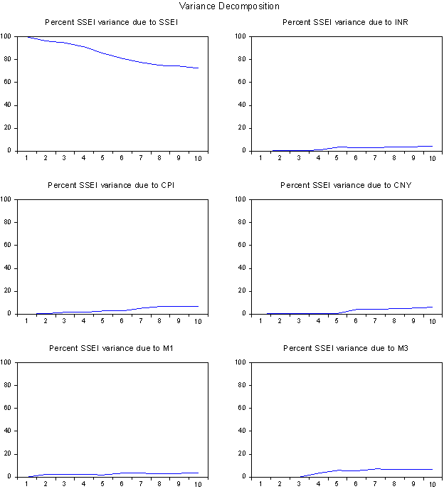

备案号:辽ICP备19007957号-1
![]() 聆听您的声音:feedback@highmark.com.cn企业热线:400-111-0321
聆听您的声音:feedback@highmark.com.cn企业热线:400-111-0321
Copyright ©2015- 海马课堂网络科技(大连)有限公司办公地址:辽宁省大连市高新技术产业园区火炬路32A号创业大厦A座18层1801室
hmkt088